12  One-way ANOVA

This chapter marks the beginning of the content you cover in Research Methods 2. You should be familiar with all the content from Research Methods 1 we covered in Chapters 1 to 11, so please revisit previous chapters if you need a refresher.

In the course materials, you have worked through manually calculating an ANOVA to gain a conceptual understanding. However, when you run an ANOVA, typically the computer does all of these calculations for you. In this chapter, we will show you how to run a one-way ANOVA using the afex package and post-hoc tests using the emmeans package.

Chapter Intended Learning Outcomes (ILOs)

By the end of this chapter, you will be able to:

• Apply and interpret a one-way ANOVA.

• Break down the results of a one-way ANOVA using post-hocs tests and apply a correction for multiple comparisons.

• Conduct a power analysis for a one-way ANOVA.

12.1 Chapter preparation

12.1.1 Introduction to the data set

For this chapter, we are using open data from experiment 2 in James et al. (2015). The abstract of their article is:

Memory of a traumatic event becomes consolidated within hours. Intrusive memories can then flash back repeatedly into the mind’s eye and cause distress. We investigated whether reconsolidation - the process during which memories become malleable when recalled - can be blocked using a cognitive task and whether such an approach can reduce these unbidden intrusions. We predicted that reconsolidation of a reactivated visual memory of experimental trauma could be disrupted by engaging in a visuospatial task that would compete for visual working memory resources. We showed that intrusive memories were virtually abolished by playing the computer game Tetris following a memory-reactivation task 24 hr after initial exposure to experimental trauma. Furthermore, both memory reactivation and playing Tetris were required to reduce subsequent intrusions (Experiment 2), consistent with reconsolidation-update mechanisms. A simple, non-invasive cognitive-task procedure administered after emotional memory has already consolidated (i.e., > 24 hours after exposure to experimental trauma) may prevent the recurrence of intrusive memories of those emotional events.

In summary, they were interested in whether you can reduce intrusive memories associated with a traumatic event. Participants were randomly allocated to one of four groups and watched a video designed to be traumatic:

1. Control

2. Reactivation + Tetris

3. Tetris

4. Reactivation

They measured the number of intrusive memories prior to the start of the study, then participants kept a diary to record intrusive memories about the film in the 7 days after watching it. The authors were interested in whether the combination of reactivation and playing Tetris would lead to the largest reduction in intrusive memories. You will recreate their analyses using a one-way ANOVA.

12.1.2 Organising your files and project for the chapter

Before we can get started, you need to organise your files and project for the chapter, so your working directory is in order.

1. In your folder for research methods and the book ResearchMethods1_2/Quant_Fundamentals, create a new folder called Chapter_12_ANOVA. Within Chapter_12_ANOVA, create two new folders called data and figures.

2. Create an R Project for Chapter_12_ANOVA as an existing directory for your chapter folder. This should now be your working directory.

3. Create a new R Markdown document and give it a sensible title describing the chapter, such as 12 ANOVA. Delete everything below line 10 so you have a blank file to work with and save the file in your Chapter_12_ANOVA folder.

4. We are working with a new data set, so please save the following data file: James_2015.csv. Right click the link and select “save link as”, or clicking the link will save the files to your Downloads. Make sure that you save the file as “.csv”. Save or copy the file to your data/ folder within Chapter_12_ANOVA.

You are now ready to start working on the chapter!

12.1.3 Activity 1 - Read and wrangle the data

As the first activity, try and test yourself by completing the following task list to practice your data wrangling skills. Create a final object called james_data to be consistent with the tasks below.

Try this

To wrangle the data, complete the following tasks:

1. Load the following packages (several of these are new, so revisit Chapter 1 if you need a refresher of installing R packages, but remember not to install packages on the university computers / online server):

   • pwr

   • effectsize

   • broom

   • afex

   • emmeans

   • performance

   • tidyverse

2. Read the data file data/James_2015.csv to the object name james_data.

3. Create a new variable called PID that equals row_number() to act as a participant ID which is currently missing from the data set.

4. Convert Condition to a factor.

5. Select and rename the following three variables as we do not need the others:

   • PID

   • Condition

   • Rename Days_One_to_Seven_Image_Based_Intrusions_in_Intrusion_Diary to intrusions.

Show me the solution

You should have the following in a code chunk:

# Load packages
library(pwr)
library(effectsize)
library(broom)
library(afex)
library(emmeans)
library(performance)
library(tidyverse)

# Read data and add new column
james_data <- read_csv("data/James_2015.csv") %>%
  mutate(PID = row_number(),
         Condition = as.factor(Condition)) %>% 
  select(PID, 
         Condition, 
         intrusions = Days_One_to_Seven_Image_Based_Intrusions_in_Intrusion_Diary)

12.1.4 Activity 2 - Create summary statistics

Next, we want to calculate some descriptive statistics to see some overall trends in the data. We are really interested in the scores from each experimental group rather than overall.

Try this

• Summarise the data to show the mean, standard deviation, and standard error for the number of intrusive memories (intrusions) grouped by Condition.

• Your table should have four columns, Condition, mean, sd, and se.

Hint: You can calculate the standard error through: sd/sqrt(n) or sd/sqrt(length(some_variable_name).

Show me the solution

You should have the following in a code chunk:

james_data %>%
  group_by(Condition) %>%
  summarise(mean = round(mean(intrusions), 2), 
            sd = round(sd(intrusions), 2), 
            se = round(sd/sqrt(length(intrusions)), 2))

Condition	mean	sd	se
1	5.11	4.23	1.00
2	1.89	1.75	0.41
3	3.89	2.89	0.68
4	4.83	3.33	0.78

12.1.5 Activity 3 - Visualisation

Now we can visualise the data. In the original paper they use a bar plot, but let’s use a better plot that gives us more information about the data.

Try this

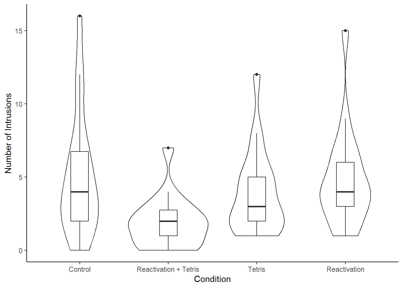
• Create a violin-boxplot with the number of intrusive memories on the y-axis and condition on the x-axis (See Chapter 7 if you need a reminder).

• Change the labels on the x-axis to something more informative for the condition names.

Your plot should look like this:

Show me the solution

You should have the following in a code chunk:

james_data %>% 
  ggplot(aes(x = Condition, y = intrusions))+
  geom_violin()+
  geom_boxplot(width = .2) + 
  scale_y_continuous(name = "Number of Intrusions") + 
  scale_x_discrete(labels = c("Control", "Reactivation + Tetris", "Tetris", "Reactivation")) + 
  theme_classic()

We can see from this plot that there are a few potential outliers in each of the groups. This information is not present in the bar plot, which is why it’s not a good idea to use them for this kind of data.

12.2 One-way ANOVA

Now we can run the one-way ANOVA using aov_ez() from the afex package and save it to the object mod. As well as running the ANOVA, the aov_ez() function also conducts a Levene’s test for homogeneity of variance so that we can test our final assumption.

12.2.1 Activity 4 - Running a one-way ANOVA using afex

aov_ez() will likely produce some messages that look like errors, do not worry about these, they are just letting you know what it’s done. Run the code below to view the results of the ANOVA.

mod <- aov_ez(id = "PID", # the column containing the participant IDs
              dv = "intrusions", # the DV 
              between = "Condition", # the between-subject variable
              es = "pes", # sets effect size to partial eta-squared
              type = 3, # this affects how the sum of squares is calculated, set this to 3
              include_aov = TRUE,
              data = james_data)

mod

Anova Table (Type 3 tests)

Response: intrusions
     Effect    df   MSE      F  ges p.value
1 Condition 3, 68 10.09 3.79 * .143    .014
---
Signif. codes:  0 '***' 0.001 '**' 0.01 '*' 0.05 '+' 0.1 ' ' 1

Just like with the t-tests and correlations, we can use tidy() to make the output easier to work with. Run the below code to transform the output. Do not worry about the warning message, it is just telling you it does not know how to automatically rename the columns so it will keep the original names.

mod_output <- mod$anova_table %>% 
  tidy()

Warning in tidy.anova(.): The following column names in ANOVA output were not
recognized or transformed: num.Df, den.Df, MSE, ges

mod_output

term	num.Df	den.Df	MSE	statistic	ges	p.value
Condition	3	68	10.08578	3.794762	0.1434073	0.0140858

• term = the IV
  
• num.Df = degrees of freedom effect
• den.Df = degrees of freedom residuals
• MSE = Mean-squared errors
• statistic = F-statistic
• ges = effect size
  
• p.value = p.value

You should refer to the lecture for more information on what each variable means and how it is calculated.

• Is the overall effect of Condition significant? Yes No

• What is the F-statistics to 2 decimal places?

• According to the rules of thumb, the effect size is Small Medium Large

12.2.2 Activity 5 - Checking assumptions for ANOVA

To test the assumptions, we must use the model we created with aov_ez(). For a one-way independent ANOVA, the assumptions are the same as for a Student t-test / regression model with a categorical predictor:

1. The DV is interval or ratio data.

2. The observations should be independent.

3. The residuals should be normally distributed.

4. There should be homogeneity of variance between the groups.

We know that 1 and 2 are met because of the design of our study. To test 3, we can look at the qq-plot of the residuals. Instead of saving just the model object, we must specifically select the aov component and run our diagnostic plots.

plot(mod$aov, 
     which = 2)

Figure 12.1: qq-plot for model residuals.

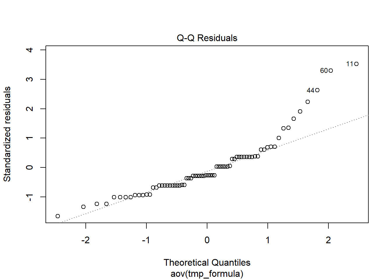
The qq-plot shows the assumption of normality might not be ideal. Is this a problem? If the sample sizes for each group are equal, then ANOVA is robust to violations of both normality and of homogeneity of variance. If you are interested, there is a good discussion of these issues in Blanca et al. (2018) and Knief & Forstmeier (2021). We can check how many participants are in each condition using count():

james_data %>% 
  count(Condition)

Condition	n
1	18
2	18
3	18
4	18

Thankfully, the sample sizes are equal, so we should be OK to proceed with the ANOVA. It is not clear whether normality was checked in the original paper.

For the last assumption, we can test homogeneity of variance by checking the third diagnostic plot for the scale against location.

plot(mod$aov, 
     which = 3)

Figure 12.2: Diagnostic plot for homogeneity of variance.

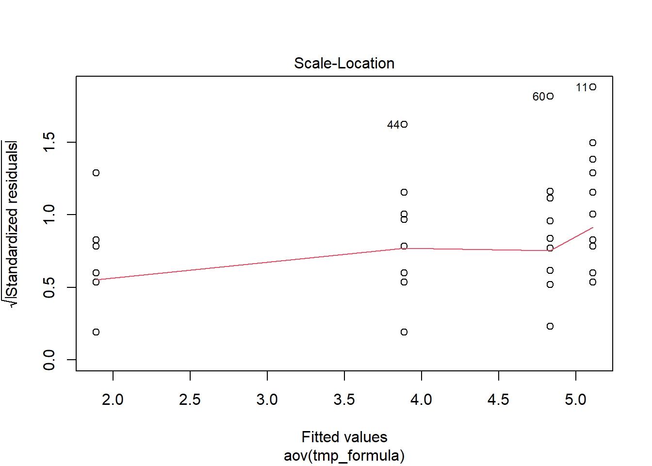
Compared to normality, this assumption looks closer to being supported as the variance of each group is approximately equal. James et al. (2015) suspect there might be issues with this assumption as they mention that the ANOVAs do not assume equal variance, however, the results of the ANOVA that are reported are identical to our results above where no correction has been made although the post-hoc tests are Welch t-tests (you can tell this because the degrees of freedom have been adjusted and are not whole numbers).

While all of this might seem very confusing - we imagine you might be wondering what the point of assumption testing is given that it seems to be ignored - we are showing you this for three reasons:

1. To reassure you that sometimes the data can fail to meet the assumptions and it is still ok to use the test. To put this in statistical terms, many tests are robust to mild deviations of normality and unequal variance, particularly with equal sample sizes.

2. As a critical thinking point, to remind you that just because a piece of research has been published does not mean it is perfect and you should always evaluate whether the methods used are appropriate.

3. To reinforce the importance of pre-registration where these decisions could be made in advance, and/or open data and code so that analyses can be reproduced exactly to avoid any ambiguity about exactly what was done. In this example, given the equal sample sizes and the difference in variance between the groups isn’t too extreme, it looks like it is still appropriate to use an ANOVA but the decisions and justification for those decisions could have been more transparent.

Note

The check_model() function from performance also works here, so you can see what it looks like if you run:

check_model(mod$aov)

12.2.3 Activity 6 - Post-hoc tests

For post-hoc comparisons, the paper appears to have computed Welch t-tests but there is no mention of any multiple comparison correction. We could reproduce these results by using t.test() for each of the contrasts.

For example, to compare condition 1 (the control group) with condition 2 (the reactivation plus tetris group) we could run:

james_data %>%
  filter(Condition %in% c("1", "2")) %>%
  droplevels() %>% # ignore unused factor levels
  t.test(intrusions ~ Condition, 
         data = .)

    Welch Two Sample t-test

data:  intrusions by Condition
t = 2.9893, df = 22.632, p-value = 0.006627
alternative hypothesis: true difference in means between group 1 and group 2 is not equal to 0
95 percent confidence interval:
 0.990331 5.454113
sample estimates:
mean in group 1 mean in group 2 
       5.111111        1.888889 

Important

Because Condition has four levels, we cannot just specify intrustion ~ Condition because a t-test compares two groups and it would not know which of the four to compare so first we have to filter the data and use a new function droplevels(). It’s important to remember that when it comes to R there are two things to consider, the data you can see and the underlying structure of that data. In the above code we use filter() to select only conditions 1 and 2 so that we can compare them. However, that does not change the fact that R “knows” that Condition has four levels - it does not matter if two of those levels do not have any observations any more, the underlying structure still says there are four groups. droplevels() tells R to remove any unused levels from a factor. Try running the above code but without droplevels() and see what happens.

However, a quicker and better way of doing this that allows you apply a correction for multiple comparisons easily is to use emmeans() which computes all possible pairwise comparison t-tests and applies a correction to the p-value.

First, we use emmeans() to run the comparisons and then we can pull out the contrasts and use tidy() to make it easier to work with.

Run the code below. Which conditions are significantly different from each other? Are any of the comparisons different from the ones reported in the paper now that a correction for multiple comparisons has been applied?

mod_pairwise <-emmeans(mod, 
                       pairwise ~ Condition, 
                       adjust = "bonferroni")

mod_contrasts <- mod_pairwise$contrasts %>% 
  tidy()

mod_contrasts

term	contrast	null.value	estimate	std.error	df	statistic	adj.p.value
Condition	Condition1 - Condition2	0	3.2222222	1.058604	68	3.0438406	0.0199179
Condition	Condition1 - Condition3	0	1.2222222	1.058604	68	1.1545602	1.0000000
Condition	Condition1 - Condition4	0	0.2777778	1.058604	68	0.2624001	1.0000000
Condition	Condition2 - Condition3	0	-2.0000000	1.058604	68	-1.8892804	0.3787128
Condition	Condition2 - Condition4	0	-2.9444444	1.058604	68	-2.7814405	0.0419783
Condition	Condition3 - Condition4	0	-0.9444444	1.058604	68	-0.8921602	1.0000000

Warning

The inquisitive among you may have noticed that mod is a list of 5 and seemingly contains the same thing three times: anova_table, aov and Anova. The reasons behind the differences are too complex to go into detail on this course (see The R Companion website here for more information) but the simple version is that anova_table and Anova use one method of calculating the results (type 3 sum of squares) and aov uses a different method (type 1 sum of squares). What’s important for your purposes is that you need to use anova_table to view the overall results (and replicate the results from papers) and aovto run the follow-up tests and to get access to the residuals (or lm() for factorial ANOVA). As always, precision and attention to detail is key.

12.2.4 Activity 7 - Power and effect sizes

Finally, we can replicate their power analysis using pwr.anova.testfrom the pwr package.

On the basis of the effect size of d = 1.14 from Experiment 1, we assumed a large effect size of f = 0.4. A sample size of 18 per condition was required in order to ensure an 80% power to detect this difference at the 5% significance level.

pwr.anova.test(k = 4, 
               f = .4, 
               sig.level = .05, 
               power = .8)

     Balanced one-way analysis of variance power calculation 

              k = 4
              n = 18.04262
              f = 0.4
      sig.level = 0.05
          power = 0.8

NOTE: n is number in each group

We have already got the effect size for the overall ANOVA, however, we should also really calculate Cohen’s d using cohens_d() from effectsize for each of the pairwise comparisons. This code is a little long because you need to do it separately for each comparison, bind them all together and then add them to mod_contrasts - just make sure your understand which bits of the code you would need to change to run this on different data. As we are binding rows and columns rather than joining, it is critical the comparisons are already in the correct order.

# Calculate Cohen's d for all comparisons
d_1_2 <- cohens_d(intrusions ~ Condition, 
                 data = filter(james_data, 
                               Condition %in% c(1, 2)) %>% 
                   droplevels())

d_1_3 <- cohens_d(intrusions ~ Condition, 
                 data = filter(james_data, 
                               Condition %in% c(1, 3)) %>% 
                   droplevels()) 

d_1_4 <- cohens_d(intrusions ~ Condition, 
                 data = filter(james_data, 
                               Condition %in% c(1, 4)) %>% 
                   droplevels())

d_2_3 <- cohens_d(intrusions ~ Condition, 
                 data = filter(james_data, 
                               Condition %in% c(2, 3)) %>% 
                   droplevels())

d_2_4 <- cohens_d(intrusions ~ Condition, 
                 data = filter(james_data, 
                               Condition %in% c(2, 4)) %>% 
                   droplevels())

d_3_4 <- cohens_d(intrusions ~ Condition, 
                 data = filter(james_data, 
                               Condition %in% c(3, 4)) %>% 
                   droplevels())

# Bind all the comparisons in the order of mod_contrasts
pairwise_ds <- bind_rows(d_1_2, 
                         d_1_3, 
                         d_1_4,
                         d_2_3, 
                         d_2_4, 
                         d_3_4)

# Bind this object to the mod_contrasts object
mod_contrasts <- mod_contrasts %>%
  bind_cols(pairwise_ds)

Warning

What are your options if the data do not meet the assumptions and it’s really not appropriate to continue with a regular one-way ANOVA? As always, there are multiple options and it is a judgement call.

1. You could run a non-parametric test, the Kruskal-Wallis for between-subject designs and the Friedman test for within-subject designs.

2. If normality is the problem, you could try transforming the data.

3. You could use bootstrapping, which is not something we will cover in this course at all.

12.3 Reporting the results of your ANOVA

The below code replicates the write-up in the paper, although has changed the Welch t-test to the pairwise comparisons from emmeans().

Second, and critically, for the 7-day diary postintervention, there was a significant difference between groups in overall intrusion frequency in daily life, F(`r mod_output$num.Df`, `r mod_output$den.Df`) = `r mod_output$statistic %>% round(2)`, p = `r mod_output$p.value %>% round(3)`, ηp2 = .`r mod_output$ges %>% round(2)`. Planned comparisons demonstrated that relative to the no-task control group, only those in the reactivation-plus-Tetris group, t(`r mod_contrasts$df[1]`) = `r mod_contrasts$statistic[1] %>% round(2)`, p = `r mod_contrasts$adj.p.value[1] %>% round(2)`, d = `r mod_contrasts$Cohens_d[1] %>% round(2)`, experienced significantly fewer intrusive memories; this finding replicated Experiment 1. The reactivation-plus-Tetris group had significantly fewer intrusive thoughts than the reactivation-only group, t(`r mod_contrasts$df[5]`) = `r mod_contrasts$statistic[5] %>% round(2)`, p = `r mod_contrasts$adj.p.value[5] %>% round(2)`, d = `r mod_contrasts$Cohens_d[5] %>% round(2)`. Further, there were no significant differences between the reactivation-plus-Tetris group and the Tetris-only group, t(`r mod_contrasts$df[4]`) = `r mod_contrasts$statistic[4] %>% round(2)`, p = `r mod_contrasts$adj.p.value[4] %>% round(2)`, d = `r mod_contrasts$Cohens_d[4] %>% round(2)`, the no-task control group and the reactivation-only group, t(`r mod_contrasts$df[3]`) = `r mod_contrasts$statistic[3] %>% round(2)`, p = `r mod_contrasts$adj.p.value[3] %>% round(2)`, or between the no-task control group and the Tetris-only group, t(`r mod_contrasts$df[2]`) = `r mod_contrasts$statistic[2] %>% round(2)`, p = `r mod_contrasts$adj.p.value[2] %>% round(2)`

If you add that code to your R Markdown document, knitting it should create the following:

Second, and critically, for the 7-day diary postintervention, there was a significant difference between groups in overall intrusion frequency in daily life, F(3, 68) = 3.79, p = 0.014, ηp2 = .0.14. Planned comparisons demonstrated that relative to the no-task control group, only those in the reactivation-plus-Tetris group, t(68) = 3.04, p = 0.02, d = 1, experienced significantly fewer intrusive memories; this finding replicated Experiment 1. Critically, as predicted by reconsolidation theory, the reactivation-plus-Tetris group had significantly fewer intrusive memories than the Tetris-only group, t(68) = -1.89, p = 0.38, d = -0.84, as well as the reactivation-only group, t(68) = -2.78, p = 0.04, d = -1.11. Further, there were no significant differences between the no-task control group and the reactivation-only group, t(68) = 0.26, p = 1, or between the no-task control group and the Tetris-only group, t(68) = 1.15, p = 1

12.4 End of chapter

Well done! You have now covered how to run a one-way ANOVA using the afex package. Linear regression models are great for their flexibility, but it is not always simple for expressing a design with several levels. Combining afex and emmeans is a powerful combination when you have categorical independent variables / predictors with several levels.

In the next chapter, we will extend this to when you have multiple independent variables and you want to investigate the interaction between them for how they affect your dependent variable / outcome.

Blanca, M. J., Alarcón, R., Arnau, J., Bono, R., & Bendayan, R. (2018). Effect of variance ratio on ANOVA robustness: Might 1.5 be the limit? Behavior Research Methods, 50(3), 937–962. https://doi.org/10.3758/s13428-017-0918-2

James, E. L., Bonsall, M. B., Hoppitt, L., Tunbridge, E. M., Geddes, J. R., Milton, A. L., & Holmes, E. A. (2015). Computer Game Play Reduces Intrusive Memories of Experimental Trauma via Reconsolidation-Update Mechanisms: Psychological Science, 26(8), 1201–1215. https://doi.org/10.1177/0956797615583071

Knief, U., & Forstmeier, W. (2021). Violating the normality assumption may be the lesser of two evils. Behavior Research Methods, 53(6), 2576–2590. https://doi.org/10.3758/s13428-021-01587-5