Until now, a large component of each chapter was dedicated to data wrangling as we must first process raw data into something tidier we can apply our visualisation or modelling steps to. In this chapter, there is no data wrangling, just functions to calculate statistical power in different ways for different tests. Before, the difficulty was in unique problems in wrangling your specific data. In power analysis, the functions are pretty straight forward to use, but deciding what inputs you use are the hard parts as they are your decisions to make.
We adapted a few components of this chapter from Bartlett & Charles (2022) and we recommend referring to this article for more information on the concepts behind statistical power. However, the article focuses on the statistics software jamovi, so this chapter focuses on power analysis using the pwr package.
Chapter Intended Learning Outcomes (ILOs)
By the end of this chapter, you will be able to:
Conduct and interpret an a priori power analysis for t-tests, correlations, and regression models.
Conduct and interpret a sensitivity power analysis for t-tests, correlations, and regression models.
Report your power analysis to make it reproducible for your reader.
10.1 Chapter preparation
10.1.1 Organising your files and project for the chapter
In contrast to previous chapters, there will be no data wrangling in this chapter, so we do not need to worry about downloading files. We will still be working around some key studies, but we will introduce them as needed. However, you will still be working in an R Markdown document, so you need to make sure your working directory is in order.
In your folder for research methods and the book ResearchMethods1_2/Quant_Fundamentals, create a new folder called Chapter_10_power.
Create an R Project for Chapter_10_power as an existing directory for your chapter folder. This should now be your working directory.
Create a new R Markdown document and give it a sensible title describing the chapter, such as 10 Statistical Power and Effect Sizes. Delete everything below line 10 so you have a blank file to work with and save the file in your Chapter_10_power folder.
In a code chunk, load the pwr and tidyverse packages. If you need to install any packages, revisit Chapter 1 if you need a refresher, but remember not to install packages on the university computers / online server.
You are now ready to start working on the chapter!
10.2 NHST and statistical power recap
Given there is no data wrangling for this chapter and the functions for power analysis are pretty straight forward, we have a little space to recap the key concepts behind power analysis. Almost all the work here comes into thinking and justifying your decisions, rather than spending lots of time on wrangling and analysis.
The branch of statistics we are using here is Null Hypothesis Significance Testing (NHST). There are two types of hypotheses and what you are trying to establish is the probability of rejecting the null hypothesis. Those two hypotheses are:
The null hypothesis which states that there is no difference (\(H_0: \mu_1 = \mu_2\)) or no relationship (\(H_0: r = 0\)).
The alternative hypothesis which states that there is a difference (\(H_1: \mu_1 \ne \mu_2\)) or there is a relationship (\(H_1: r \ne 0\)).
NHST is designed to control error rates associated with two main decisions around these hypotheses:
Type I error - or false positive, is the probability of rejecting the null hypothesis when it should not be rejected (otherwise called alpha or \(\alpha\)). In other words, you conclude that there is a real “effect” when in fact there is no effect. The field standard rate of acceptable false positives is \(\alpha = .05\), meaning that we would accept 1 in 20 studies may be a false positive.
Type II error - or false negative, is the probability of retaining the null hypothesis when it should be rejected (otherwise called beta or \(\beta\)). In other words, you conclude that there was no real “effect” when in fact there was one. There is less tradition around this, but the most common rule of thumb you will come across is \(\beta = .20\), meaning that we would accept 1 in 5 studies may be a false negative.
Statistical power is the opposite of beta and represents the long-run probability of correctly rejecting the null hypothesis when there is a real effect to detect. In other words, how likely are you to detect an effect that is really there? You calculate Power as \(1-\beta\), meaning that if the field standard for beta is \(\beta = .20\), then the field standard for power is \(1 - .20 = .80\) (80%).
In addition to alpha and beta/power, there are two other key concepts (there are more depending on the test, but we will add them in when we need them):
Effect size - A number that expresses the magnitude of the phenomenon relevant to your research question. In Chapters 8 and 9, we introduced you to different standardised effect sizes such as Pearson’s r and Cohen’s d.
Sample size - The number of observations (usually participants, but it might be animals or stimuli depending on your topic) in your study.
Critically, there is a relationship between these four concepts, where if you know three, you can calculate the fourth in a process called power analysis. The two most useful types of power analysis are:
A priori power analysis: How many participants do I need, for a given alpha, beta/power, and smallest effect size of interest? This is most useful in the design stage to help you plan how many participants you need to design an informative study.
Sensitivity power analysis: What effect size can I detect, for a given alpha, beta/power, and sample size? This is most useful after you finish collecting data or when you are using secondary data as the sample size is not longer under your control and it helps put your findings in context.
You may now be thinking though, if there is a relationship between all four concepts, could we calculate power for a given alpha, sample size, and effect size? It is a tempting idea and you might see some articles report it, but unfortunately is is misleading and tells you nothing more than the p-value does. The short version is we are typically using a sample to learn something about a population, so there is uncertainty in the estimate. Using the observed effect size in your study assumes this is the true population effect, which is rarely a good assumption. If you are interested, Lakens (2022) is a great resource for sample size justification in general, but also explains why post-hoc power is not a good idea.
After the brief recap, we will now focus on a priori and sensitivity power analyses applied to different statistical models.
10.3 Power analysis for t-tests / categorical predictors
10.3.1 Introduction to the study
In this section, imagine we are designing a study to build on Irving et al. (2022) who tested an intervention to correct statistical misinformation. Participants read an article about a new fictional study where one passage falsely concludes watching TV causes cognitive decline. In the correction group, participants receive an extra passage where the fictional researcher explains they only reported a correlation, not a causal relationship. In the no-correction group, the extra passage just explains the fictional researcher was not available to comment. Irving et al. then tested participants’ comprehension of the story and coded their answers for mistaken causal inferences. They expected participants in the correction group to make fewer causal inferences than those in the no-correction group, and found evidence supporting this prediction with an effect size equivalent to Cohen’s d = 0.64, 95% CI = [0.28, 0.99]. Inspired by their study, we want to design an experiment to correct another type of misinformation in articles.
Irving et al. (2022) themselves provide an excellent example of explaining and justifying the rationale behind their power analysis, so we will walk through the decision making process and how it changes the outputs. For our smallest effect size of interest, our starting point is the estimate of d = 0.64. However, it is worth consulting other sources to calibrate our understanding of effects in the area, such as Irving et al. citing a meta-analysis. For debunking, the average effect across 30 studies was d = 1.14, 95% CI = [0.68, 1.61], so we could use the lower bound of the confidence interval, but this may still represent an overestimate. Irving et al. used the smallest effect (d = 0.54) from the studies most similar to their design which was included in the meta-analysis. As a value slightly smaller than the other estimates, we will also use this as the smallest effect of interest for our study.
Now we have settled on our smallest effect size of interest, we will use d = 0.54 in the following demonstrations. We start with a priori and sensitivity power analysis for two independent samples, exploring how the outputs change as we alter inputs like alpha, power, and the number of tails in the test.
10.3.2 A priori power analysis
For an independent samples t-test (we will cover regression shortly), there is the function pwr.t.test(). We can enter the following arguments:
n: The number of observations.
d: The effect size as Cohen’s d.
sig.level: The alpha level.
power: The power value as 1-\(\beta\).
type: Whether you want power for a one-, paired-, or independant-samples t-test.
alternative: Whether you have a one- or two-sided hypothesis.
Remember, power analysis works by leaving one argument blank, so for calculating the sample size, we leave n blank or enter NULL as the argument. As our starting point, we enter d = 0.54, sig.level = .05, power = .90, type = two.sample and alternative = two-sided.
pwr.t.test(n =NULL, d =0.54, sig.level = .05, power = .90, type ="two.sample", alternative ="two.sided")
     Two-sample t test power calculation

              n = 73.04123
              d = 0.54
      sig.level = 0.05
          power = 0.9
    alternative = two.sided

NOTE: n is number in *each* group
As the note warns us, for an independent-samples t-test, n represents the number of observations per group, so we need 74 per group (we round up as we cannot have .04 of a person) or N = 148.
If you wanted to use these values in inline code, you can save the power analysis object and pick out values to work with.
irving_samplesize <-pwr.t.test(n =NULL, d =0.54, sig.level = .05, power = .90, type ="two.sample", alternative ="two.sided") %>%pluck("n") %>%ceiling()
In this code, we save the power analysis function to an object, use the pluck() function to pick out a specific component (the argument name must be spelt exactly), and use the ceiling() function to round up. This helps to avoid manually calculating the values as you can use the object.
# sample size per groupirving_samplesize# total sample sizeirving_samplesize *2
[1] 74
[1] 148
The power analysis function is pretty straight forward to work with, it is the thinking and decision making that goes into selecting the value for each argument that is the hardest part here. It is ultimately a subjective decision you must be able to justify in a report and there will always be compromises. You never have unlimited resources, so you are trying to balance designing the most informative study with maximizing the resources available to you.
Try this
With decision making in mind, we can tweak the arguments to see how it affects the sample size we need. We will tweak one argument at a time, so your starting point will be the arguments we started with above.
If we used a one-tailed test predicting a positive effect ("greater"), we would need participants per group (N = ).
If we wanted to make fewer type I errors and reduce alpha to .005, we would need participants per group (N = ).
If we were happy with a larger beta and reduce power to .80 (80%), we would need participants per group (N = ).
If we wanted to decrease our smallest effect size of interest and set d = .40, we would need participants per group (N = ).
If we thought it was appropriate to change the design to within-subjects and use a paired-samples t-test instead ("paired"), we would need participants.
Show me the solution
We can calculate sample size for a one-tailed test by entering alternative = "greater" or alternative = "less". This must match the effect size direction or you will receive an error.
pwr.t.test(n =NULL, d =0.54, sig.level = .05, power = .90, type ="two.sample", alternative ="greater") %>%pluck("n") %>%ceiling()
[1] 60
We can decrease alpha by entering alpha = .005 to calculate the sample size for reducing the type I error rate.
pwr.t.test(n =NULL, d =0.54, sig.level = .005, power = .90, type ="two.sample", alternative ="two.sided") %>%pluck("n") %>%ceiling()
[1] 117
We can decrease power if we were happy with a larger beta / type II error rate by entering power = .80.
pwr.t.test(n =NULL, d =0.54, sig.level = .05, power = .80, type ="two.sample", alternative ="two.sided") %>%pluck("n") %>%ceiling()
[1] 55
We can decrease the smallest effect size of interest if we wanted the study to be more sensitive by entering d = .40.
pwr.t.test(n =NULL, d =0.40, sig.level = .05, power = .90, type ="two.sample", alternative ="two.sided") %>%pluck("n") %>%ceiling()
[1] 133
If we changed the design and test to within-subjects, we can enter type = "paired".
pwr.t.test(n =NULL, d =0.54, sig.level = .05, power = .90, type ="paired", alternative ="two.sided") %>%pluck("n") %>%ceiling()
[1] 39
These are important lessons to recognise which inputs increase and which decrease the sample size you need. For an a priori power analysis in the design phase, you can tweak the inputs depending on how sensitive you want your study given the resources available to you. Holding everything else constant, we can summarise the patterns as:
Using a one-tailed test the sample size you need.
Reducing alpha the sample size you need.
Reducing power / increasing beta the sample size you need.
Reducing the smallest effect size of interest the sample size you need.
Switching to a within-subjects design the sample size you need.
10.3.3 Sensitivity power analysis
Now imagine you already knew the sample size or had access to a population of a known size. In this scenario, you would conduct a sensitivity power analysis. This would tell you what effect sizes your study would be powered to detect for a given alpha, power, and sample size. This is helpful for interpreting your results as you can outline what effect sizes your study was sensitive to and which effects would be too small for you to reliably detect.
Imagine we had finished collecting data and we knew we had 40 participants in each group but did not conduct an a priori power analysis when designing the study. Instead of leaving n blank, we can leave d blank.
pwr.t.test(n =40, d =NULL, sig.level = .05, power = .90, type ="two.sample", alternative ="two.sided")
     Two-sample t test power calculation

              n = 40
              d = 0.7339255
      sig.level = 0.05
          power = 0.9
    alternative = two.sided

NOTE: n is number in *each* group
The output tells us that the study is sensitive to detect effect sizes of d = 0.73 with 90% power. This helps us to interpret the results if we did not plan with power in mind. If the effect size we could detect with 90% power is larger than our smallest effect size of interest, our study was potentially underpowered. This might sound like post-hoc power we warned you about, but the key difference is you are comparing the effect size your study was sensitive to against your smallest effect size of interest, not your observed effect size.
For a sensitivity power analysis, you will often find yourself with unequal sample sizes. The previous function assumes equal sample sizes, but pwr.t2n.test() lets you set n1 and n2. For example, imagine we ended up with two groups of 39 and 43 participants.
pwr.t2n.test(n1 =39, n2 =43,d =NULL, sig.level = .05, power = .90, alternative ="two.sided") %>%pluck("d") %>%round(digits =2)
[1] 0.73
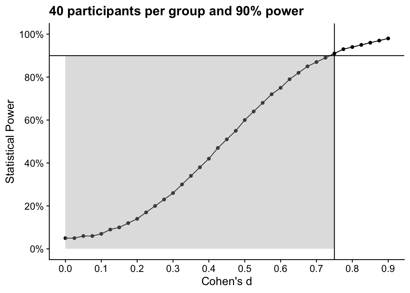
One other key point here is power exists along a curve, there is not just a single value for power once your sample size is fixed. We can visualise this through something called a power curve. Figure 10.1 shows statistical power against Cohen’s d as the effect size for a fixed sample of 40 participants per group. We would have 90% power to detect a Cohen’s d of 0.75 (the value is a little different here as we set the effect size, rather than calculate it as the output), shown where the two lines meet. You would have more and more power to detect effects larger than 0.75 (follow the curve to the right), but less power to detect effects smaller than 0.75 (follow the curve to the left). The grey shaded region highlights the effects your study would be less sensitive to than your desired value for power.
Figure 10.1: Power curve for 40 participants per group and 90% power.
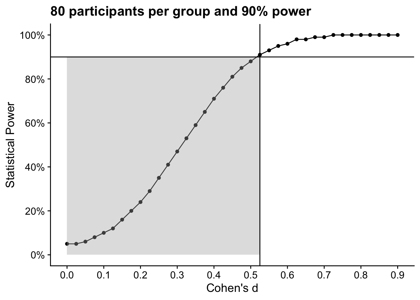
On the other hand, Figure 10.2 shows statistical power against Cohen’s d as the effect size for a fixed sample of 80 participants per group. This time, we would have 90% power to detect effects of d = 0.53 and there is a smaller grey region. We would have more power to detect effects larger than d = 0.53 but less power to detect effects smaller than 0.53.
Figure 10.2: Power curve for 80 participants per group and 90% power.
Hopefully, these demonstrations reinforce the idea of sensitivity and how power exists along a curve once you have a fixed sample size.
10.3.4 Power for regression with a categorical predictor
In Chapters 8 and 9, we recommended expressing your designs as linear regression models. They have many benefits, but one downside is the effect size and process we need for power analysis is not the most intuitive. Typically, people report effect sizes like Cohen’s d when comparing groups, but here we need Cohen’s \(f^2\). You can convert between effect sizes and we recommend the website psychometrica.de which has an online calculator for converting effect sizes in section 14. Alternatively, you can use the following code to save \(f^2\) as an object.
# enter your Cohen's d valued <-0.54# This calculates f2 from df2 <- (d /2)^2
Now we have \(f^2\), we can use the function pwr.f2.test() which calculates power for regression models. For the equivalent of a t-test, we have the following new arguments:
u: The numerator degrees of freedom, the number of predictors in your model.
v: The denominator degrees of freedom, a little more awkward but the sample size minus u minus 1.
f2: The effect size \(f^2\), which is a kind of transformed version of \(R^2\) for the amount of variance explained by the model.
For our power analysis, we will save the inputs as objects to make it easier to reuse them, and enter them in the following arguments:
# number of predictorsu <-1# alpha for type I error ratealpha <- .05# power for 1-betapower <- .90pwr.f2.test(u = u, v =NULL, sig.level = alpha, power = power, f2 = f2)
     Multiple regression power calculation

              u = 1
              v = 144.0824
             f2 = 0.0729
      sig.level = 0.05
          power = 0.9
Using the objects from the power analysis, we can calculate the sample size we need with a little reorganising.
irving_v <-pwr.f2.test(u =1, v =NULL, sig.level = .05, power = .90, f2 = f2) %>%pluck("v") ceiling(irving_v + u +1)
[1] 147
In the t-test power analysis function, we needed 148 participants in total, so this is off by 1 participant. There are a few steps for rounding errors here, so this is close enough to show it is the equivalent but more awkward process.
If you wanted to use this function for a sensitivity power analysis, you can convert \(f^2\) back to Cohen’s d using psychometrica.de or use the following code:
# f2 from the outputf2 <- .073# convert to d by square root of f2 times 2d <-sqrt(f2) *2
10.4 Power analysis for correlations / continuous predictors
10.4.1 Introduction to the study
For this section, we need a new study to work with for a correlation / continuous predictor. Wingen et al. (2020) were interested in the relationship between the replication rate in psychology studies and the public trust in psychology research. The replication crisis has led to a lot of introspection in the field to consider how we conduct robust research. However, being honest about the state of the field might be good for science, but perhaps it is related to lower public trust in science. We will focus on study 1 which asked the question: does trust in psychology correlate with expected replicability?
Wingen et al. (2020) reported a power analysis and they aimed for 95% power, 5% alpha, and their smallest effect size of interest was r = .20. Like Irving et al. (2022), they chose this value based on a meta-analysis which summarised hundreds of studies across social psychology. We will use these values as a starting point and adapt them to see it’s impact on the sample size we need.
10.4.2 A priori power analysis
For Pearson’s r correlation, there is the function pwr.r.test(). All the arguments are the same as for the t-test, apart from we specify r as an effect size instead of Cohen’s d and we do not need to specify the type of test.
pwr.r.test(n =NULL, r = .20, sig.level = .05, power = .95, alternative ="two.sided")
     approximate correlation power calculation (arctangh transformation)

              n = 318.2637
              r = 0.2
      sig.level = 0.05
          power = 0.95
    alternative = two.sided
As before, we can isolate the sample size we would need for a study sensitive to these inputs.
pwr.r.test(n =NULL, r = .20, sig.level = .05, power = .95, alternative ="two.sided") %>%pluck("n") %>%ceiling()
[1] 319
Our starting point is 319 participants to detect our smallest effect size of interest r = .20 with 95% power and 5% alpha.
Try this
With decision making in mind, we can tweak the arguments to see how it affects the sample size we need. We will tweak one argument at a time, so your starting point will be the arguments we started with above.
If we used a one-tailed test predicting a positive relationship, we would need participants. This reproduces the power analysis from Wingen et al., as they used a one-tailed test.
If we wanted to make fewer type I errors and reduce alpha to .005, we would need participants.
If we were happy with a larger beta and reduce power to .80 (80%), we would need participants.
Show me the solution
We can calculate sample size for a one-tailed test by entering alternative = "greater" or alternative = "less". This must match the effect size direction or you will receive an error.
pwr.r.test(n =NULL, r = .20, sig.level = .05, power = .95, alternative ="greater") %>%pluck("n") %>%ceiling()
[1] 266
We can decrease alpha by entering alpha = .005 to calculate the sample size for reducing the type I error rate.
pwr.r.test(n =NULL, r = .20, sig.level = .005, power = .95, alternative ="two.sided") %>%pluck("n") %>%ceiling()
[1] 485
We can decrease power if we were happy with a larger beta / type II error rate by entering power = .80.
pwr.r.test(n =NULL, r = .20, sig.level = .05, power = .80, alternative ="two.sided") %>%pluck("n") %>%ceiling()
[1] 194
Like for the independent samples t-test, the design phase allows you to carefully consider the inputs you choose and tweak them depending on how sensitive you want your study given the resources available to you. Holding everything else constant, we can summarise the patterns here as:
Using a one-tailed test the sample size you need.
Reducing alpha the sample size you need.
Reducing power / increasing beta the sample size you need.
10.4.3 Sensitivity power analysis
Wingen et al. (2020) is a great example of a sensitivity power analysis in the wild as they are relatively rare to see in published research. They explain they recruited participants online, so they ended up with more participants than they aimed for.
Try this
Their final sample size was 271, so try and adapt the function to calculate the effect size r they were sensitive to. Both of these answers assume 5% alpha and a one-sided test.
To 2 decimal places, they could detect an effect of r = with 80% power and r = with 95% power.
Show me the solution
You should have had this in a code chunk for 80% power:
pwr.r.test(n =271, r =NULL, sig.level = .05, power = .80, alternative ="greater") %>%pluck("r") %>%round(digits =2)
[1] 0.15
And this in a code chunk for 95% power:
pwr.r.test(n =271, r =NULL, sig.level = .05, power = .95, alternative ="greater") %>%pluck("r") %>%round(digits =2)
[1] 0.2
10.4.4 Power for regression with a continuous predictor
Like the categorical predictor, we have a mismatch between the effect size you typically see reported (Pearson’s r) and the effect size we need for a regression power analysis (\(f^2\)). The website psychometrica.de still works for converting effect sizes in section 14. Alternatively, you can use the following code to save \(f^2\) as an object.
# effect size as Pearson's rr <- .20# convert to f2 by squaring r valuesf2 <- r^2/ (1- r^2)
Now we have \(f^2\), we can use the function pwr.f2.test() which calculates power for regression models.
# number of predictorsu <-1# alpha for type I error ratealpha <- .05# power for 1-betapower <- .95pwr.f2.test(u = u, v =NULL, sig.level = alpha, power = power, f2 = f2)
     Multiple regression power calculation

              u = 1
              v = 311.807
             f2 = 0.04166667
      sig.level = 0.05
          power = 0.95
Using the objects from the power analysis, we can calculate the sample size we need with a little reorganising.
wingen_v <-pwr.f2.test(u =1, v =NULL, sig.level = .05, power = .95, f2 = f2) %>%pluck("v") ceiling(wingen_v + u +1)
[1] 314
In the Pearson’s r power analysis function, we needed 319 participants in total, so the estimate is off by 5 participants this time. We still have a few steps for rounding error, so this is close enough to show it is the equivalent but more awkward process.
If you wanted to use this function for a sensitivity power analysis, you can convert \(f^2\) back to Pearson’s \(r\) using psychometrica.de or use the following code:
# f2 from the outputf2 <- .042# convert to r from the square root of f2 / f2 + 1r <-sqrt(f2 / (f2 +1))
10.5 Reporting a power analysis
Bakker et al. (2020) warned that only 20% of power analyses contained enough information to be fully reproducible. To report your power analysis, the reader needs the following four key pieces of information:
The type of test you based the power analysis on (e.g., t-test, correlation, regression),
The software used to calculate power (i.e., cite the pwr package, see How to cite R),
The inputs that you used (alpha, power, effect size, sample size, tails), and
Why you chose those inputs.
In this chapter, we will only cover the first three. The justification for your inputs comes under evaluation skills, so we will work on that in the course materials. Please note there is no single ‘correct’ way to report a power analysis, we just provide examples. Just be sure that you have the four key pieces of information.
10.5.1 Reporting a t-test power analysis
For a t-test, the key distinctive input is Cohen’s d as the effect size.
“To detect an effect size of Cohen’s d = 0.54 with 90% power (alpha = .05, two-tailed), the pwr package (Champely, 2020) in R (R Core Team, 2024) suggests we would need 74 participants per group (N = 148) for an independent samples t-test.”
Alternatively, if you reported a sensitivity power analysis, the emphasis goes to the effect size your study would be sensitive to.
“With our final sample size of 40 participants per group, a sensitivity power analysis for an independent samples t-test using the pwr package (Champely, 2020; R Core Team, 2024) showed we could detect an effect size of d = 0.73 with 90% power (5% alpha, two-sided).”
10.5.2 Reporting a correlation power analysis
For a correlation, the key distinctive input is Pearson’s r as the effect size.
“To detect an effect size of r = .20 with 95% power (alpha = .05, one-tailed), the pwr package (Champely, 2020) in R (R Core Team, 2024) suggests we would need 266 participants for a Pearson’s r correlation.”
And for a sensitivity power analysis.
“With our final sample size of 271 participants, a sensitivity power analysis for a Pearson’s r correlation using the pwr package (Champely, 2020; R Core Team, 2024) showed we could detect an effect size of r = .20 with 95% power (5% alpha, one-sided).”
10.5.3 Reporting a regression power analysis
For regression, the key distinctive inputs are \(f^2\) as the effect size, including any details of converting effect sizes, plus the number of predictors.
“To detect an effect size of Cohen’s \(f^2\) = .073, we first converted the effect size from d = 0.54. For 90% power (alpha = .05, two-tailed), the pwr package (Champely, 2020) in R (R Core Team, 2024) suggests we would need 147 participants split into two groups for a regression model with one categorical predictor.”
For a sensitivity power analysis, remember to include a note of any effect size conversions.
“We used the pwr package (Champely, 2020; R Core Team, 2024) to conduct a sensitivity power analysis for linear regression with one predictor. With a final sample size of 319, we would be able to detect an effect size of Cohen’s \(f^2\) = .041 (95% power, 5% alpha). Converted to Pearson’s r, this would be an effect size of r = .20.”
10.6 Test Yourself
To end the chapter, we have some knowledge check questions to test your understanding of the concepts we covered in the chapter. We then have some error mode tasks to see if you can find the solution to some common errors in the concepts we covered in this chapter.
10.6.1 Knowledge check
Question 1. If you want to conduct an a priori power analysis , what input do you leave blank to solve for?
Question 2. If you want to conduct a sensitivity power analysis , what input do you leave blank to solve for?
Read the following output for an a priori power analysis. The next two questions are based on this output.
     Two-sample t test power calculation

              n = 89.95986
              d = 0.42
      sig.level = 0.05
          power = 0.8
    alternative = two.sided

NOTE: n is number in *each* group
Question 3. Our smallest effect size of interest is:
Question 4. For these inputs, we would need to recruit how many participants per group?
Read the following output for a sensitivity power analysis. The next two questions are based on this output.
     approximate correlation power calculation (arctangh transformation)

              n = 72
              r = 0.3695127
      sig.level = 0.05
          power = 0.9
    alternative = two.sided
Question 5. Our final sample size was:
Question 6. For these inputs, what effect size would we be sensitive to detect?
10.6.2 Error mode
The following questions are designed to introduce you to making and fixing errors. For this topic, we focus on simple linear regression between two continuous variables. There are not many outright errors that people make here, more misspecifications that are not doing what you think they are doing.
Create and save a new R Markdown file for these activities. Delete the example code, so your file is blank from line 10. Create a new code chunk to load the packages tidyverse and pwr.
Below, we have several variations of a code chunk error or misspecification. Copy and paste them into your R Markdown file below the code chunk to load tidyverse and pwr. Once you have copied the activities, click knit and look at the error message you receive. See if you can fix the error and get it working before checking the answer.
unconverted effect sizes
Question 7. Copy the following code chunk into your R Markdown file and press knit. You should get a cryptic sounding error like Error in uniroot(function(n) eval(p.body) - power, c(4 + 1e-10, 1e+09)): f() values at end points not of opposite sign.
```{r}pwr.r.test(n =NULL, r = .20, sig.level = .05, power = .95, alternative ="less")```
Explain the solution
In this example, we specified a positive effect size but negative one-tailed test. They must be consistent, so you either need to make the hypothesis the same:
pwr.r.test(n =NULL, r = .20, sig.level = .05, power = .95, alternative ="greater")
Or the effect size the same:
pwr.r.test(n =NULL, r =-.20, sig.level = .05, power = .95, alternative ="less")
Both will produce the same sample size as it is the absolute effect which is important, but we recommend making it consistent with your research question / hypothesis.
Question 8. Copy the following code chunk into your R Markdown file and press knit. You want to conduct a sensitivity power analysis when you have unequal sample sizes. You should get the following error: Error in pwr.t.test(n1 = 40, n2 = 50, d = NULL, sig.level = 0.05, power = 0.9, : unused arguments (n1 = 40, n2 = 50).
```{r}pwr.t.test(n1 =40, n2 =50,d =NULL, sig.level = .05, power = .90, alternative ="two.sided")```
Explain the solution
In this example, we used the wrong function. pwr.t.test() only accepts n as a single argument. If you want a sensitivity power analysis for unequal sample sizes, you need the function pwr.t2n.test():
pwr.t2n.test(n1 =40, n2 =50,d =NULL, sig.level = .05, power = .90, alternative ="two.sided")
Question 9. Copy the following code chunk into your R Markdown file and press knit. In your research to establish your smallest effect size of interest, you found a meta-analysis which found the average effect size for your topic was d = 0.54. For your correlational study, you use this effect size for your a priori power analysis. This…works, but is this all consistent?
```{r}pwr.r.test(n =NULL, r = .54, sig.level = .05, power = .95, alternative ="two.sided")```
Explain the solution
In this example, we used the wrong effect size. We see this error a lot when people are looking for past studies to inform their smallest effect size of interest. You find a meta-analysis which is perfect, but it reports Cohen’s d when you want Pearson’s r for your study. You can convert between effect sizes (with the caveat the studies should be comparable), but the same number means different things. Mistaking d = 0.54 for Pearson’s r is going to vastly underestimate the sample size you need, as it would be converted to r = .26.
pwr.r.test(n =NULL, r = .26, sig.level = .05, power = .95, alternative ="two.sided")
10.7 Words from this Chapter
Below you will find a list of words that were used in this chapter that might be new to you in case it helps to have somewhere to refer back to what they mean. The links in this table take you to the entry for the words in the PsyTeachR Glossary. Note that the Glossary is written by numerous members of the team and as such may use slightly different terminology from that shown in the chapter.
(stats) The cutoff value for making a decision to reject the null hypothesis; (graphics) A value between 0 and 1 used to control the levels of transparency in a plot
A number between 0 and 1 where 0 indicates impossibility of the event and 1 indicates certainty
10.8 End of Chapter
Great work, being able to conduct a power analysis is a great skill to have for designing an informative study. Although things have improved over the years, it is still relatively rare to see a study in the wild report a power analysis to justify their sample size. Keep in mind they involve a lot of subjective decision making as the values you choose for alpha, power, and your smallest effect size have flexibility. A larger sample - and hence more powerful study - would always be useful, but you are never working with unlimited resources. You must make compromises and think about whether you can conduct an informative study with the resources available to you. This means the hard work comes into making decisions about the values you enter, rather than the data skills for power analysis being difficult.
In the next - and final for the Research Methods 1 component - chapter, we cover screening data and decision making in data analysis. In Chapters 8 and 9, we covered topics like diagnostic checks for statistical models. Some of them looked fine, whereas some looked potentially problematic. In the next chapter, we work through the decisions you must make when analysing data like checking for missing data, outliers, and issues with diagnostic checks. Importantly, we outline the kind of solutions you can consider for those problems which we omitted in previous chapters.
Bakker, M., Veldkamp, C. L. S., Akker, O. R. van den, Assen, M. A. L. M. van, Crompvoets, E., Ong, H. H., & Wicherts, J. M. (2020). Recommendations in pre-registrations and internal review board proposals promote formal power analyses but do not increase sample size. PLoS ONE, 15(7), e0236079. https://doi.org/10.1371/journal.pone.0236079
Bartlett, J., & Charles, S. (2022). Power to the People: ABeginner’s Tutorial to PowerAnalysis using jamovi. Meta-Psychology, 6. https://doi.org/10.15626/MP.2021.3078
Irving, D., Clark, R. W. A., Lewandowsky, S., & Allen, P. J. (2022). Correcting statistical misinformation about scientific findings in the media: Causation versus correlation. Journal of Experimental Psychology. Applied. https://doi.org/10.1037/xap0000408
R Core Team. (2024). R: A language and environment for statistical computing. R Foundation for Statistical Computing. https://www.R-project.org/
Wingen, T., Berkessel, J. B., & Englich, B. (2020). No Replication, NoTrust? HowLowReplicabilityInfluencesTrust in Psychology. Social Psychological and Personality Science, 11(4), 454–463. https://doi.org/10.1177/1948550619877412