2 Creating Reproducible Documents
In this chapter, we introduce you to using code to create reproducible research. Creating reproducible research means you will write text and code that completely and transparently performs an analysis from start to finish in a way that produces the same result for different people using the same software on different computers. We will cover things such as file structure and setting a working directory, using R Markdown files, and writing code chunks.
As well as improving transparency with others researchers, reproducible research benefits you. When you return to an analysis or task after days, weeks, or months, you will thank past you for doing things in a transparent, reproducible way, as you can easily pick up right where you left off.
Chapter Intended Learning Outcomes (ILOs)
By the end of this chapter, you will be able to:
Understand and set your working directory, either manually or through creating an R project.
Create a knit an R Markdown file to create a reproducible document.
Use inline code to combine text and code output in your reproducible documents.
Identify and fix common errors in knitting R Markdown files.
2.1 File structure, working directories, and R Projects
In chapter 1, we never worked with files, so you did not have to worry about where you put things on your computer. Before we can start working with R Markdown files, we must explain what a working directory is and how your computer knows where to find things.
Your working directory is the folder where your computer starts to look for files. It would be able to access files from within that folder and within sub-folders in your working directory, but it would not be able to access folders outside your working directory.
In this course, we are going to prescribe a way of working to support an organised file system, helping you to know where everything is and where R will try to save things on your computer and where it will try to save and load things. Once you become more comfortable working with files, you can work in a different way that makes sense to you, but we recommend following our instructions for at least RM1 as the first course.
2.1.1 Activity 1: Create a folder for all your work
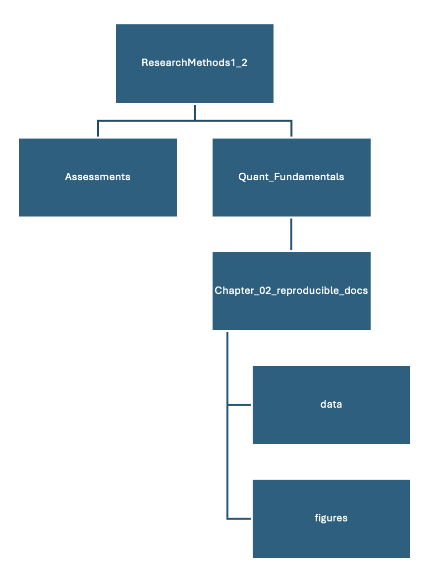
In your documents or OneDrive, create a new folder called ResearchMethods1_2. This will be your highest level folder where you will save everything for Research Methods 1 and 2.
Top tip
When you are a student at the University of Glasgow, you have access to the full Microsoft suite of software. One of those is the cloud storage system OneDrive. We heavily recommend using this to save all your work in as it backs up your work online and you can access it from multiple devices.
Within that folder, create two new folders called Assessments and Quant_Fundamentals. In Assessments, you can save all your assessments for RM1 and RM2 as you come to them. In Quant_Fundamentals, that is where you will save all your work as you progress through this book.
Within Quant_Fundamentals, create a new folder called Chapter_02_reproducible_docs. As you work through the book, you will create a new chapter folder each time you start a new chapter and the sub-folders will always be the same. Within Chapter_02_reproducible_docs, create two new folders called data and figures. As a diagram, it should look like Figure 2.1.
How to name files and folders
You might notice in the folder names we avoided using spaces by adding things like underscores _ or capitalising different words. Historically, spaces in folder/file names could cause problems for code, but now it’s just slightly easier when file names and folder names do not have spaces in them.
For naming files and folders, try and choose something sensible so you know what it refers to. You are trying to balance being as short as possible, while still being immediately identifiable. For example, instead of fundamentals of quantitative analysis, we called it Quant_Fundamentals.
Warning
When you create and name folders to use with R / RStudio, whatever you do, do not call the folder “R”. If you do this, sometimes R has an identity crisis and will not save or load your files properly. It can also really damage your setup and require you to reinstall everything as R tends to save all the packages in a folder called R. If there is another folder called R, then it gets confused and stops working properly.
File management when using the online server
If we support you to use the online University of Glasgow R Server, working with files is a little different. If you downloaded R / RStudio to your own computer or you are using one of the library/lab computers, please ignore this section.
The main disadvantage to using the R server is that you will need create folders on the server and then upload and download any files you are working on to and from the server. Please be aware that there is no link between your computer and the R server. If you change files on the server, they will not appear on your computer until you download them from the server, and you need to be very careful when you submit your assessment files that you are submitting the right file. This is the main reason we recommend installing R / RStudio on your computer wherever possible.
Going forward throughout this book, if you are using the server, you will need to follow an extra step where you also upload them to the sever. As an example:
Log on to the R server using the link we provided to you.
In the file pane, click
New folderand create the same structure we demonstrated above.Download
ahi-cesd.csvandparticipant-info.csvinto thedatafolder you created for chapter 2. To download a file from this book, right click the link and select “save link as”. Make sure that both files are saved as “.csv”. Do not open them on your machine as often other software like Excel can change setting and ruin the files.Now that the files are stored on your computer, go to RStudio on the server and click
UploadthenBrowseand choose the folder for the chapter you are working on.Click
Choose fileand go and find the data you want to upload.
2.1.2 Manually setting the working directory
Now that you have a folder structure that will keep everything nice and organised, we will demonstrate how you can manually set the working directory. If you open RStudio, you can check where the current working directory is by typing the function getwd() into the console and pressing enter/return. That will show you the current file path R is using to navigate files. If you look at the Files window in the bottom right, this will also show you the files and folders available from your working directory.
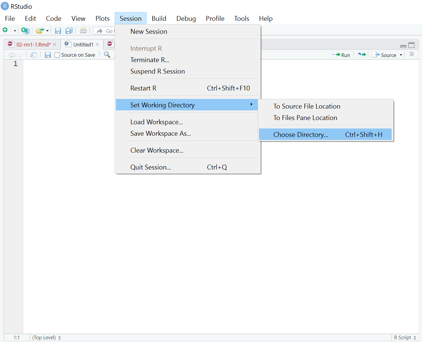
If you click on the top menu Session >> Set Working Directory >> Choose Directory..., (Figure 2.2) you can navigate through your documents or OneDrive until you can select Chapter_02_reproducible_docs. Click open and that will set the folder as your working directory. You can double check this worked by running getwd() again in the console.
2.1.3 Activity 2 - Creating an R Project
Knowing how to check and manually set your working directory is useful, but there is a more efficient way of setting your working directory alongside organised file management. You are going to create something called an R Project.
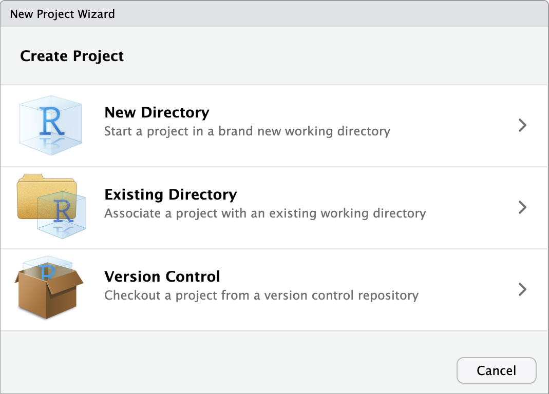
To create a new project for the work you will do in this chapter (Figure 2.3):
Click on the top menu and navigate to
File >> New Project....You have the option to select from New Directory, Existing Directory, or Version Control. You already created a folder for
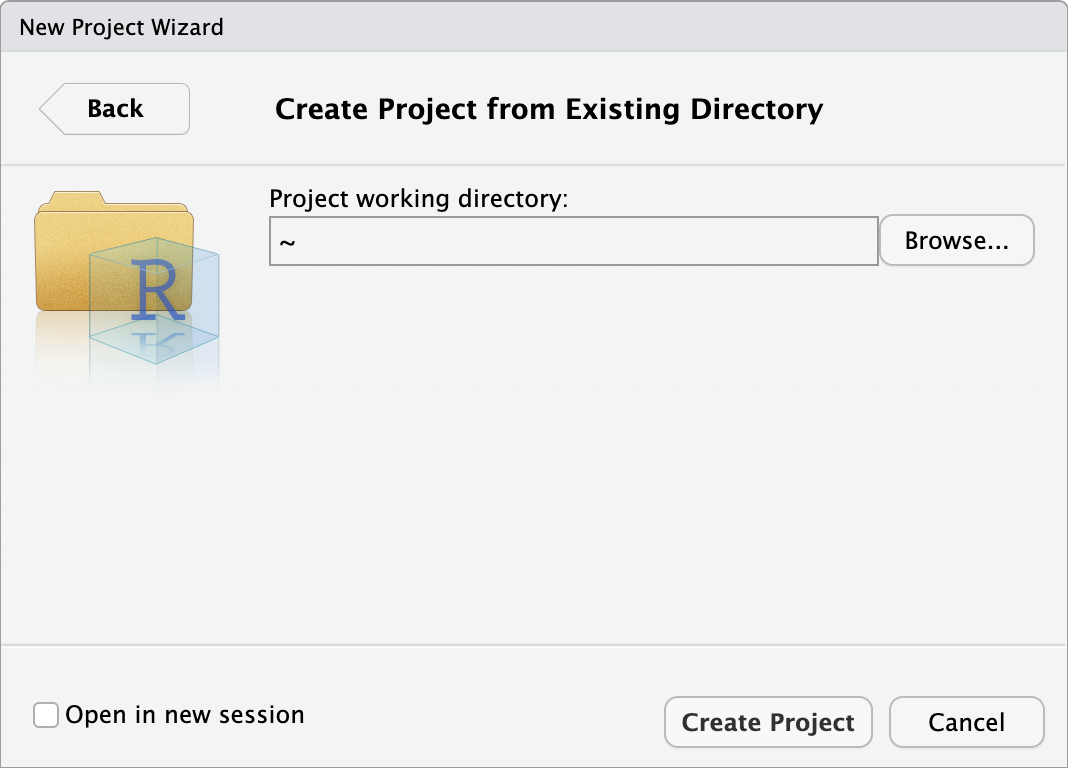
Chapter_02_reproducible_docs, so select Existing Directory.Click Browse… next to Project working directory to select the folder you want to create the project in.
When you have navigated to
Chapter_02_reproducible_docsfor this chapter, click Open and then Create Project.
RStudio will restart itself and open with this new project directory as the working directory. You should see something like Figure 2.4.
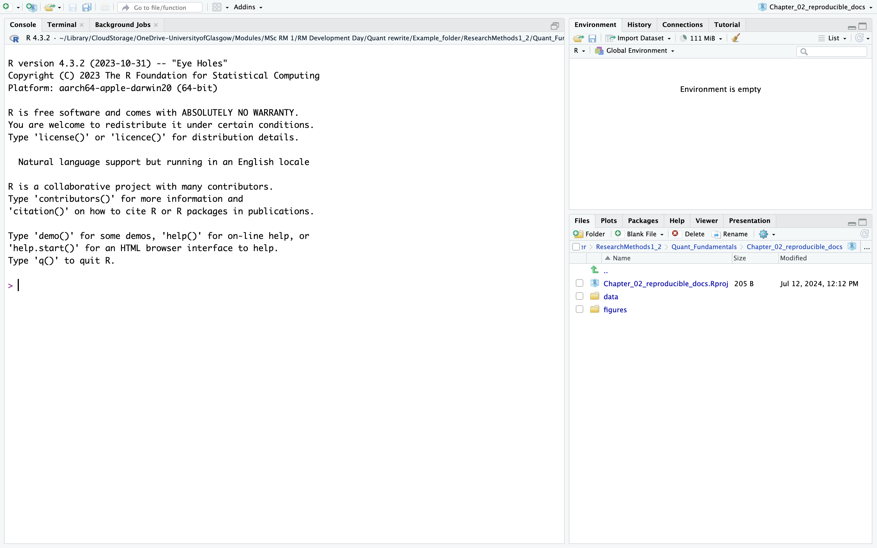
In the files tab in the bottom right window, you will see all the contents in your project directory. You can see your two sub-folders for data and figures and a file called Chapter_02_reproducible_docs.Rproj. This is a file that contains all of the project information. When you come back to this project after closing down RStudio, if you double click on the .Rproj file, it will open up your project and have your working directory all set up and ready to go.
Warning
In each chapter, we will repeat these instructions at the start to prescribe this file structure, but when you create your own folders and projects, do not ever save a new project inside another project. This can cause some hard to resolve problems. For example, it would be fine to create a new project within the Quant_Fundamentals folder as we will do for each new chapter, but should never create a new project within the Chapter_02_reproducible_docs folder.
2.2 Creating and navigating R Markdown documents
Now you know how to navigate files and folders on your computer, we can start working with R Markdown files.
Throughout this data skills book and related assignments, you will use a file format called R Markdown (abbreviated as .Rmd) which is a great way to create dynamic documents combining regular text and embedded code chunks.
R Markdown documents are self-contained and fully reproducible, meaning if you have the necessary data, you should be able to run someone else’s analyses. This is an important part of your open science training as one of the reasons we teach data skills this way is that it enables us to share open and reproducible information.
Using these worksheets enables you to keep a record of all the code you write as you progress through this book (as well as any notes to help yourself), for data skills assessments we can give you a task to add required code, and in your research reports you can independently process, visualise, and analyse your data all from one file.
For more information about R Markdown, feel free to have a look at their main webpage http://rmarkdown.rstudio.com, but for now the key advantage to know about is that it allows you to write code into a document, along with regular text, and then knit it to create your document as either a webpage (html), a PDF, or Word document (.docx).
2.2.1 Activity 3: Open, save, and knit a new R Markdown document
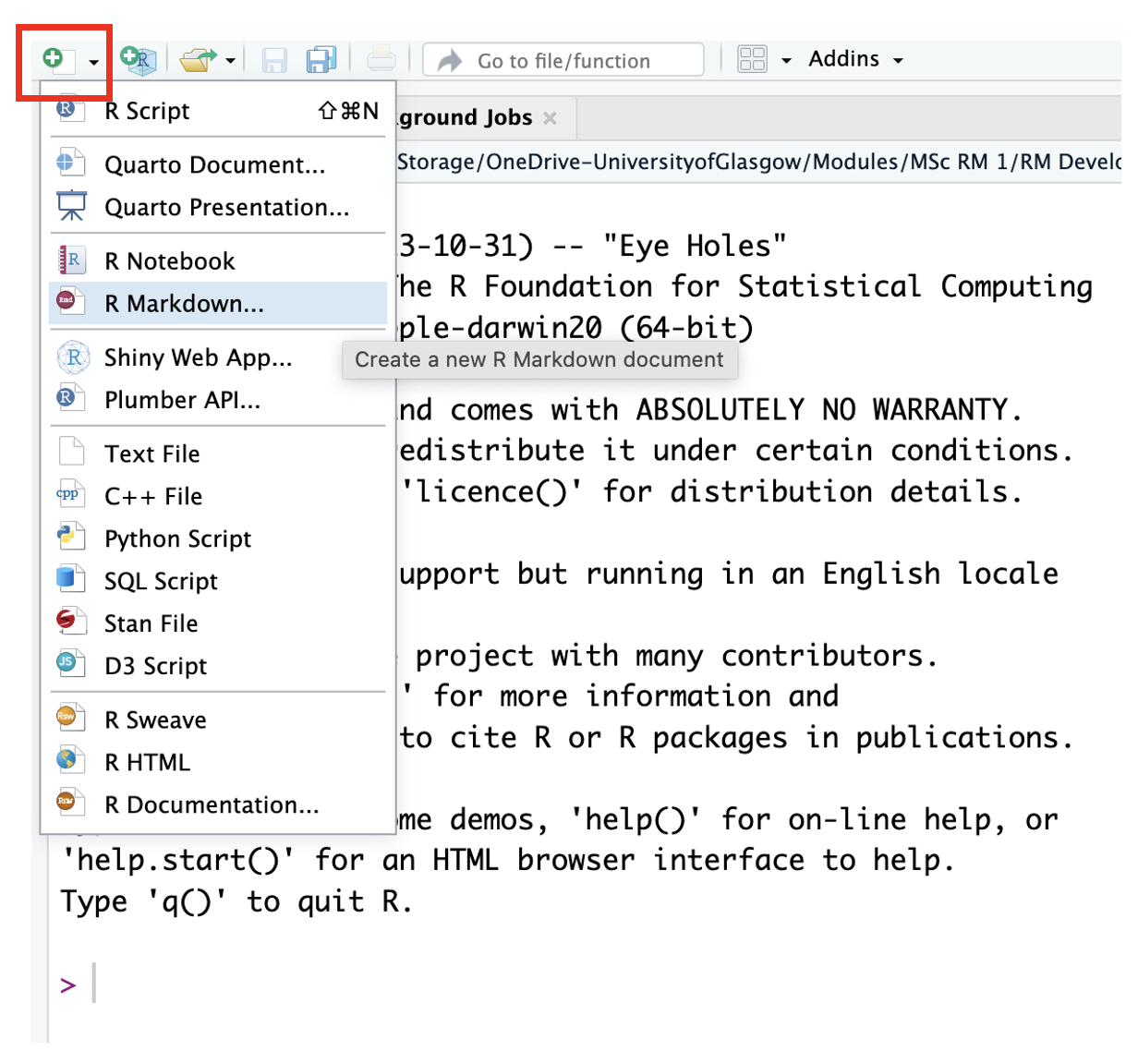
Open a new R Markdown document by clicking the ‘new item’ icon and then click ‘R Markdown’ like Figure 2.5.
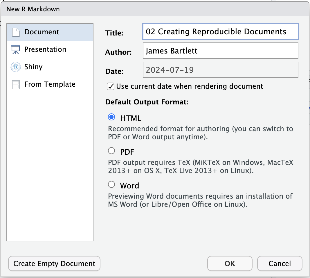
After selecting R Markdown, there are different format options you can explore in time, but Select Document and there are four boxes to complete:
Title: This is the title for the document which will appear at the top of the page. For this chapter, enter
02 Creating Reproducible Documents.Author: This is where you can add your name or names for multiple people. For this chapter, enter your GUID as this will be good practice for the data skills assignments.
Date: By default, it adds today’s date, so it will update every time you knit the document. Leave the default so you know when you completed the chapter, but if you untick, you can manually enter a static date.
Default Output Format: You have the option to select from html, PDF, and Word. We will demonstrate how to change output format in a later chapter, so keep html for now as it’s the most flexible format.
Once you click OK, this will open a new R Markdown document.
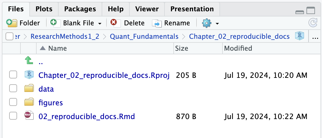
Save this R Markdown document by clicking File >> Save as from the top menu, and name this file “02_reproducible_docs”. Note the document title and file name are separate, so you still have to name the file when you save it.
If you have set the working directory correctly, you should now see this file appear in your Files window in the bottom right hand corner like Figure 2.6, alongside your .Rproj file and two folders.
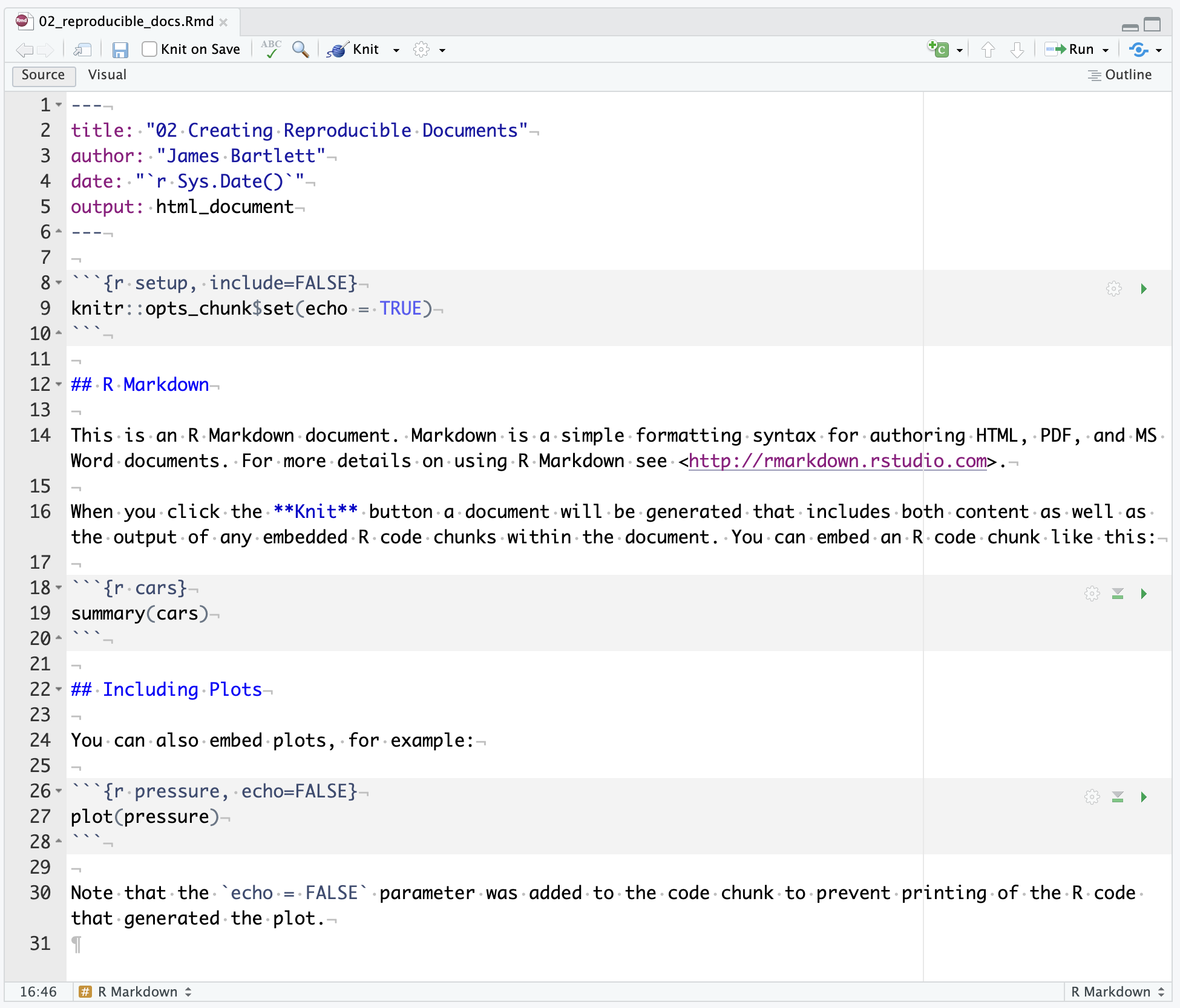
Now you have the default version of the R Markdown file, you have a bunch of text and code to show its capabilities (Figure 2.7).
We will now demonstrate what it looks like to knit a document. This means that we are going to compile (i.e., turn) our code into a document that is more presentable. This way, you can check it knits and there are no errors. So, as we add changes in the following activities, you can identify if and when any errors appear and fix them quicker.
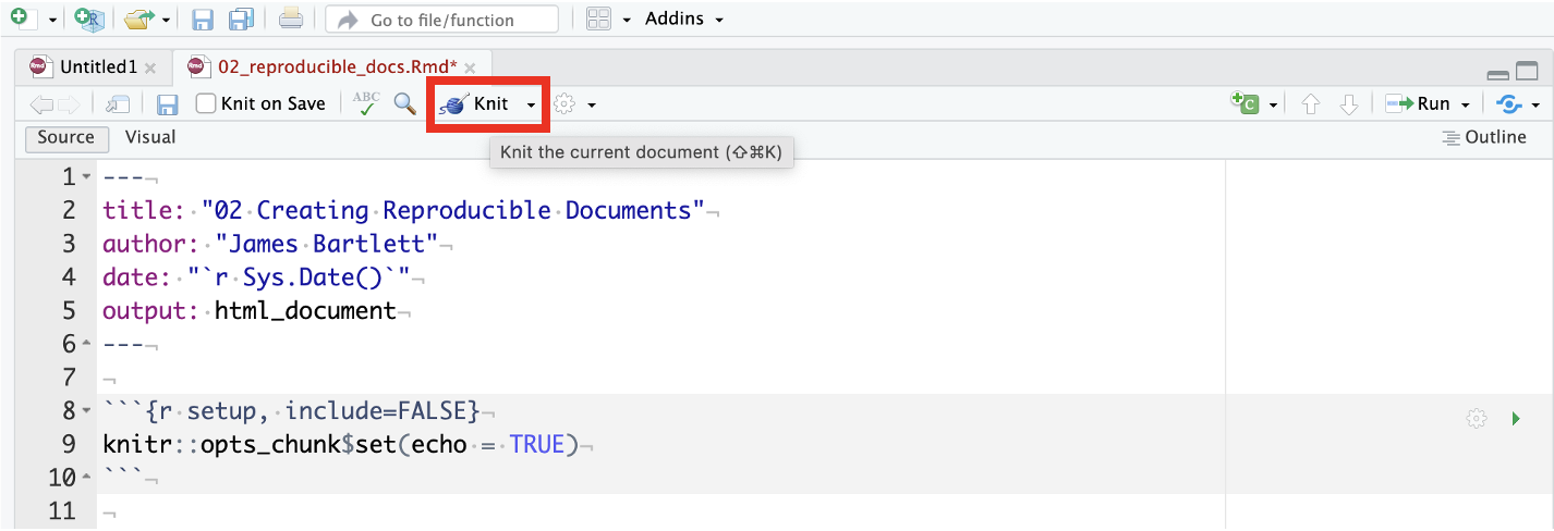
At the top of your R Markdown window, you should see a Knit button next to a little ball of yarn (Figure 2.8). If you click that, the document will knit and produce a html file.
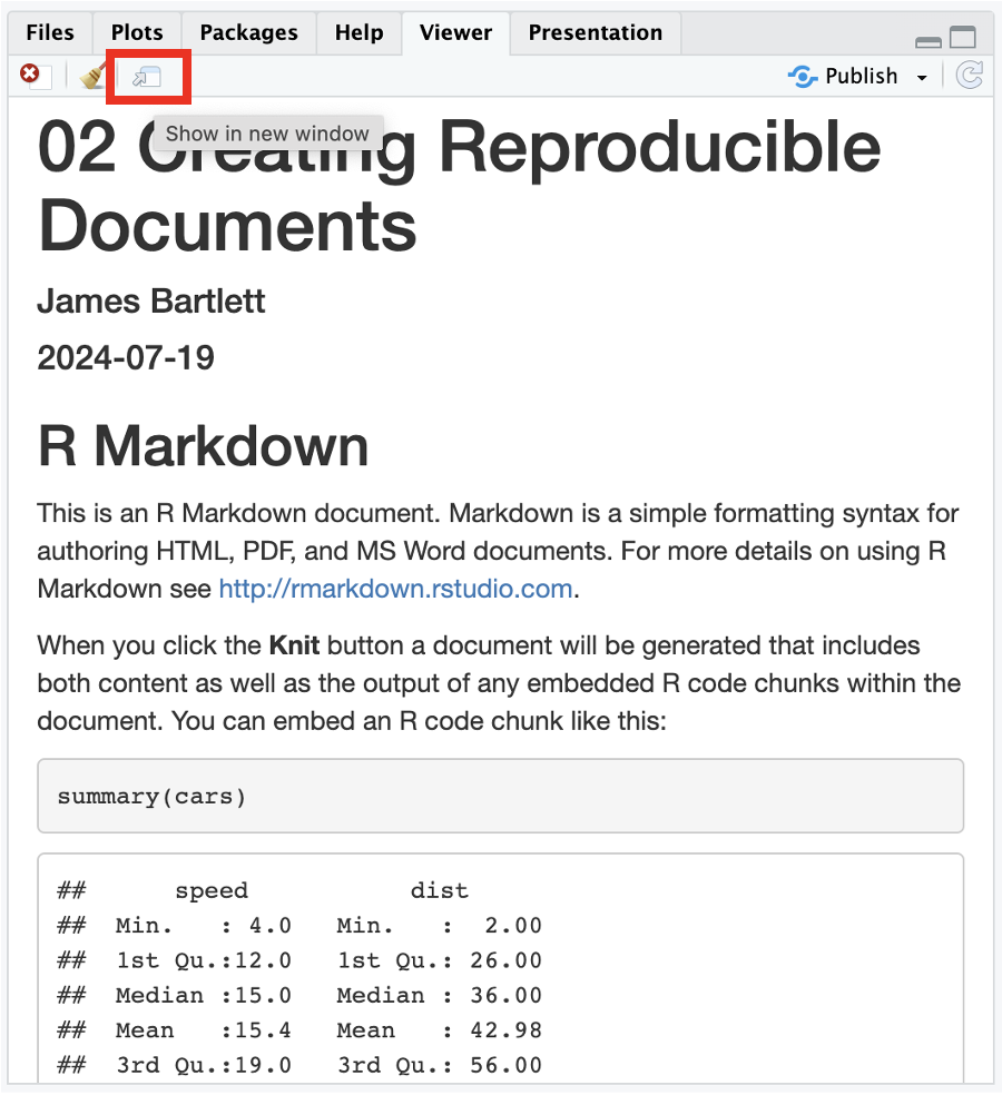
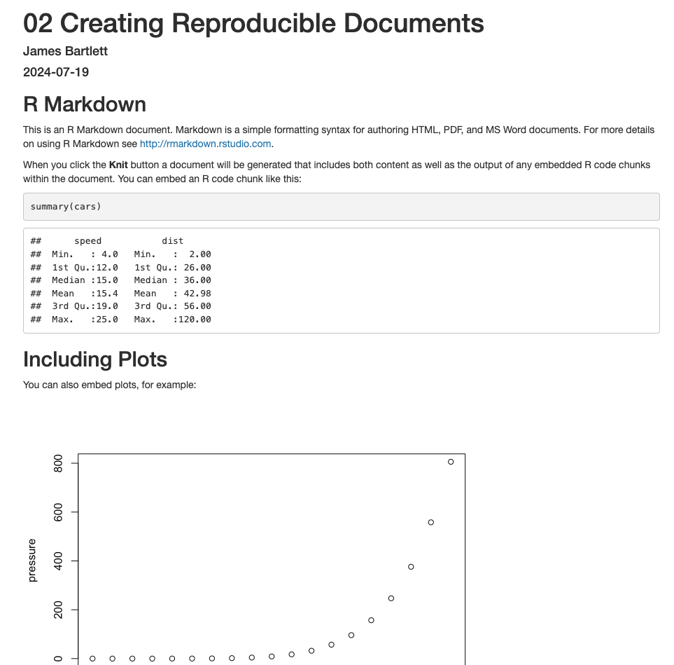
You will see a small version of the knitted document appear in the Viewer tab in the bottom right of your screen. You will also see it has created a new file in your working directory. It will have the same name as your R Markdown file, but with .html as the file ending. You can view the knitted document by clicking the “Show in new window” button or opening the file from your folder (Figure 2.9). This should open the document in your default internet browser as websites are created in html.
Now everything is working and knitting, we can start editing the R Markdown file to add new content.
2.2.2 Activity 4: Create a new code chunk
Let’s start using your new R Markdown document to combine code and text. Follow these steps:
- Delete everything below line 10.
What does the {r setup} chunk do?
At the moment, you do not need to worry about the code chunk between lines 8 and 10. We are slowly introducing you to different features in R Markdown as it’s easier to understand by doing, rather than giving you a list of explanations.
If you are really curious though, this setting forces R Markdown to show both the code and output for all code chunks. When we add code shortly, if you change it to echo = FALSE, it will only show the output and not the code.
On line 12, type “## About me”.
With your cursor on line 14, insert a blank code chunk by clicking on the top menu
Code >> Insert Chunkor using the shortcut at the top of the R Markdown window that looks like a small green c and select R.
Your document should now look something like Figure 2.10.
![]()
What you have created is called a code chunk. R Markdown assumes anything written outside of a code chunk is just normal text, just like you would have in a text editor like Word. It assumes anything written inside the code chunk is R code. This makes it easy to combine both text and code in one document.
Error mode
When you create a new code chunk, you should notice that the grey box starts and ends with three back ticks (```), followed by the {r}, and then it ends with three back ticks again. This is the structure that creates a code chunk. You could actually just type this structure instead of using the Insert approach but we are introducing you to some shortcuts
One common mistake is to accidentally delete one or more of these back ticks. A useful thing to notice is that code chunks tend to have a different color background - in the default appearance of RStudio a code chunk is grey and the normal text is white. You can use this to look for mistakes. If the colour of certain parts of your Markdown does not look right, check that you have not deleted the backticks.
Remember it is backticks (i.e. this `) and not single quotes (i.e. not this ’).
Markdown language
When you typed “## About me”, you might notice the two hashes. You will see the effect of this shortly, but this is using Markdown language to add document formatting. Markdown is a type of formatting language, so instead of using buttons to add features like you would in Word, you add symbols which will produce different features when you knit the document.
The hashes create headers. One (#) creates a first level header (larger text), two (##) creates a second level header, and so on. Make sure there is a space between the text and hash or it will not knit properly.
As we progress through the book, we will slowly introduce you to different Markdown features, but you can see the RStudio Markdown Basics page if you are interested.
2.2.3 Activity 5: Write some code
Now we are going to use the code examples you read about in Chapter 1 - Introduction to programming with R/R Studio - to add some code to our R Markdown document.
In your code chunk, write the code below but replace the values of name/age/birthday with your own details). Remember that the four lines of code should all be inside the code chunk.
Note: Text and dates need to be contained in quotation marks, e.g., “my name”. Numerical values are written without quotation marks, e.g., 45.
Error mode
Missing and/or unnecessary quotation marks are a common cause of code not working. For example, if you try and type name <- James, R will try and look for an object called James and throw an error since there is not an object called that. When you add quotation marks, R recognises you are storing a character.
2.2.4 Activity 6: Run your code
We now have code in our code chunk and now we are going to run the code. Running the code just means making it do what you told it, such as creating objects or using functions. Remember you need to write the code first, then tell RStudio to run the code.
When you are working in an R Markdown document, there are several ways to run your lines of code.
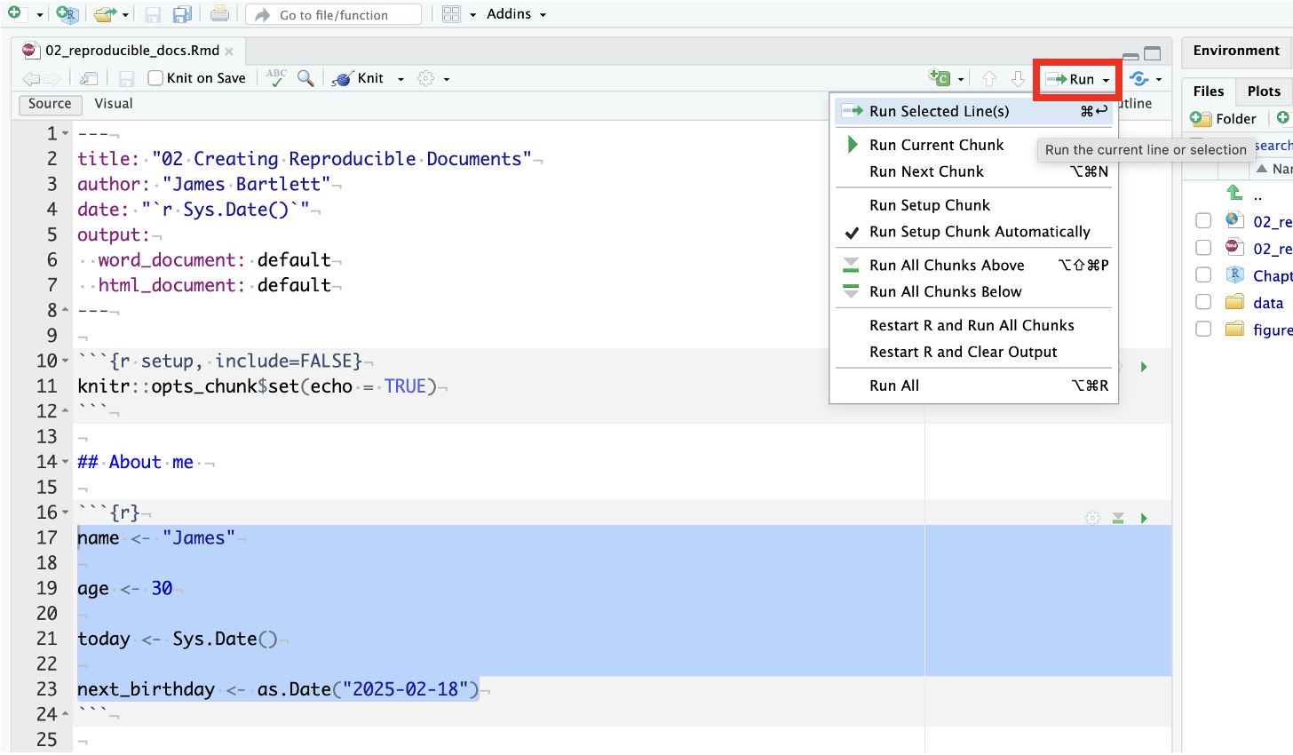
- One option is you can highlight the code you want to run and then click
Run >> Run Selected Line(s)(Figure 2.11).
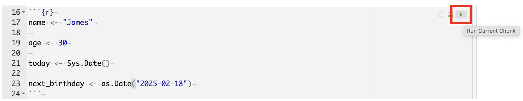
- You can press the green “play” button at the top-right of the code chunk and this will run all lines of code in that chunk (Figure 2.12).
- There are keyboard shortcuts to run code which will be the fastest as you learn and use RStudio more frequently. For example, to run a single line of code, make sure that the cursor is in the line of code (it can be anywhere on the line) you want to run and press
ctrl + enter(command + returnon a Mac).
Keyboard shortcuts
There are loads of keyboard shortcuts, but you might only use a handful to speed up your day-to-day tasks. For a full list, look in the top menu Help >> Keyboard shortcuts help.
Now run your code using one of the methods above. You should see the variables name, age, today, and next_birthday appear in the environment pane in the top right corner.
Try this
Clear out the environment using the broom handle approach we saw in Chapter 1 and try a different method to see which works best for you.
2.2.5 Activity 7: Inline code
Your code works and you now know how to run it, but one of the incredible benefits we said about R Markdown is that you can mix text and code. Even better is the ability to combine code with text to put specific outputs of your code, like a value, using inline code.
Think about a time you have had to copy and paste a value or text from one file into another and you will know how easy it can be to make mistakes or find the origin of your mistake. Inline code avoids this. It is easier to show you what inline code does rather than to explain it so let us have a go.
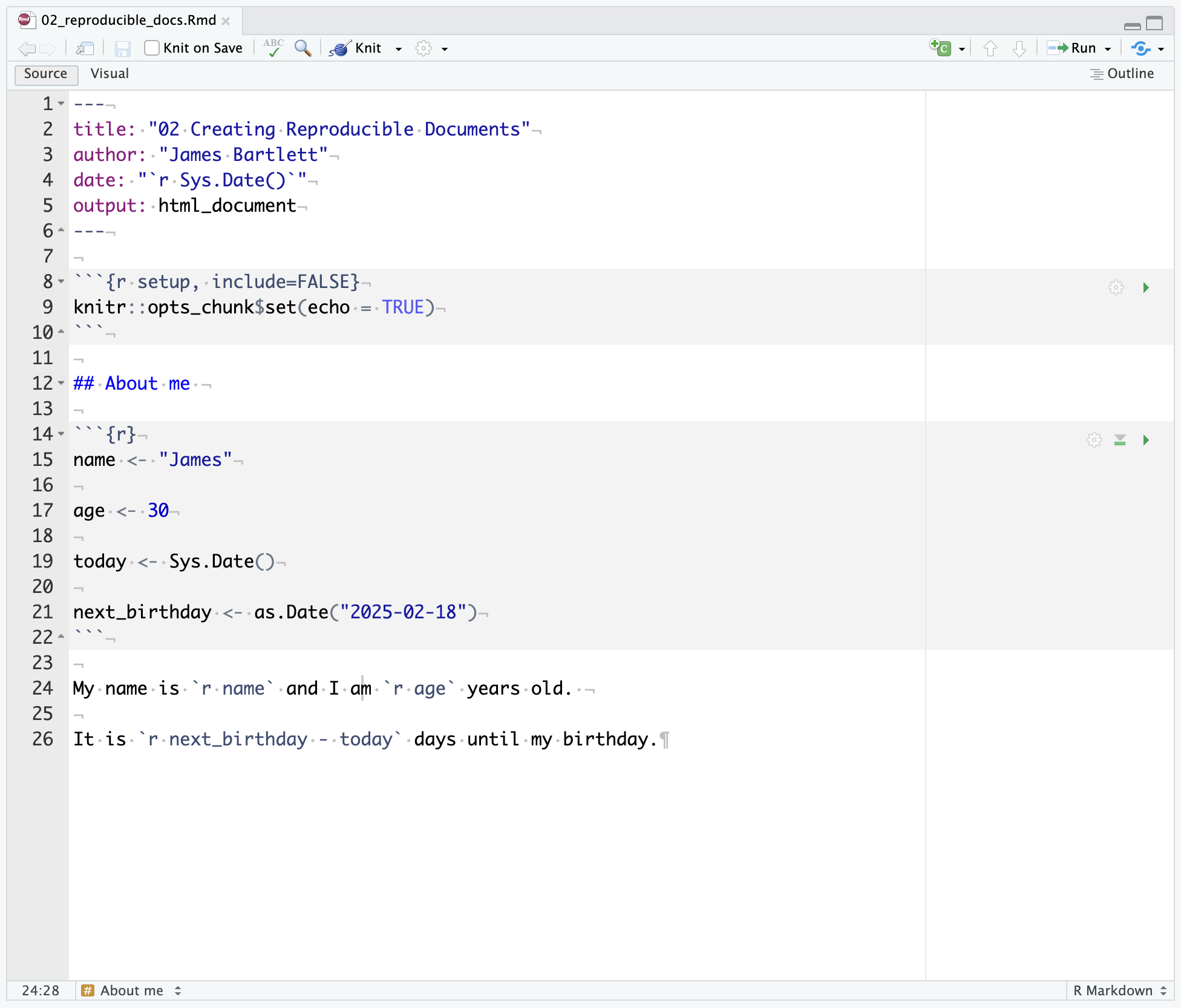
First, copy and paste this text exactly (do not change anything) to underneath and outside your code chunk:
Your .Rmd should look like Figure 2.13 but nothing will happen yet. Unlike code chunks, you cannot run inline code. You need to knit your document for it to do it’s magic.
How does inline code work?
Inline code has the following form:
or
Here, we are using the first version where we are referencing an object we already created. This is normally a good idea if you have a long function to run as it’s easier to spot mistakes in a code chunk than inline code.
You will see it has the form of a backtick (`), r and a space, the object/function you want to reference, and a final backtick. When the R Markdown file knits, it sees the r and recognises it as inline code and uses the object or function.
If you just write the two backticks without the r, it will just add code formatting and not produce inline code.
2.2.6 Activity 8: Knitting your file
As our final step in this part, we are going to knit our file again to see how it looks now. So, click the Knit button to regenerate your knitted .html version.
If you look at the knitted .html document in the Viewer tab or in your browser, you should see the sentence we copied in from Activity 7. As if by magic, that slightly odd bit of text you copied and pasted now appears as a normal sentence with the values pulled in from the objects you created:
My name is James and I am 30 years old.
It is 202 days until my birthday.
R Markdown is an incredibly powerful and flexible format, we wrote this whole book using it! There are a few final things to note about knitting that will be useful going forward for your data skills learning and assessments:
R Markdown will only knit if your code works. If you have an error, it will stop and tell you to fix the error before you can click knit and try again. This is a good way of checking whether you have written functioning code in your assessments.
When you knit an R Markdown document, it runs the code from the start of the document to the end in order, and in a fresh session. This means it cannot access your environment, just the objects you create within that R Markdown. One common error can be writing and running code as you work on the document, but the code chunks are in the wrong order, or you created an object in the console but not in the code chunks. This means R Markdown would not know the object exists yet, or it does not have access to it at all.
You can choose to knit to a Word document rather than HTML. This can be useful for sharing with others or adding further edits, but you might lose some functionality. By default, html looks good and is accessible, so that will be our default throughout this book, but look out for our instructions on what output format we want your assessments in.
You can choose to knit to PDF, however, unless you are using the server this requires a LaTeX installation and can be quite complicated. If you do not already know what LaTeX is and how to use it, we do not recommend trying to knit to PDF just yet. If you do know how to use LaTeX, you probably do not need us to give you instructions!
We will test some of these warnings in error mode in the test yourself section, but we have one final demonstration for how R Markdown files support reproducibility.
2.3 Demonstrating reproducibility
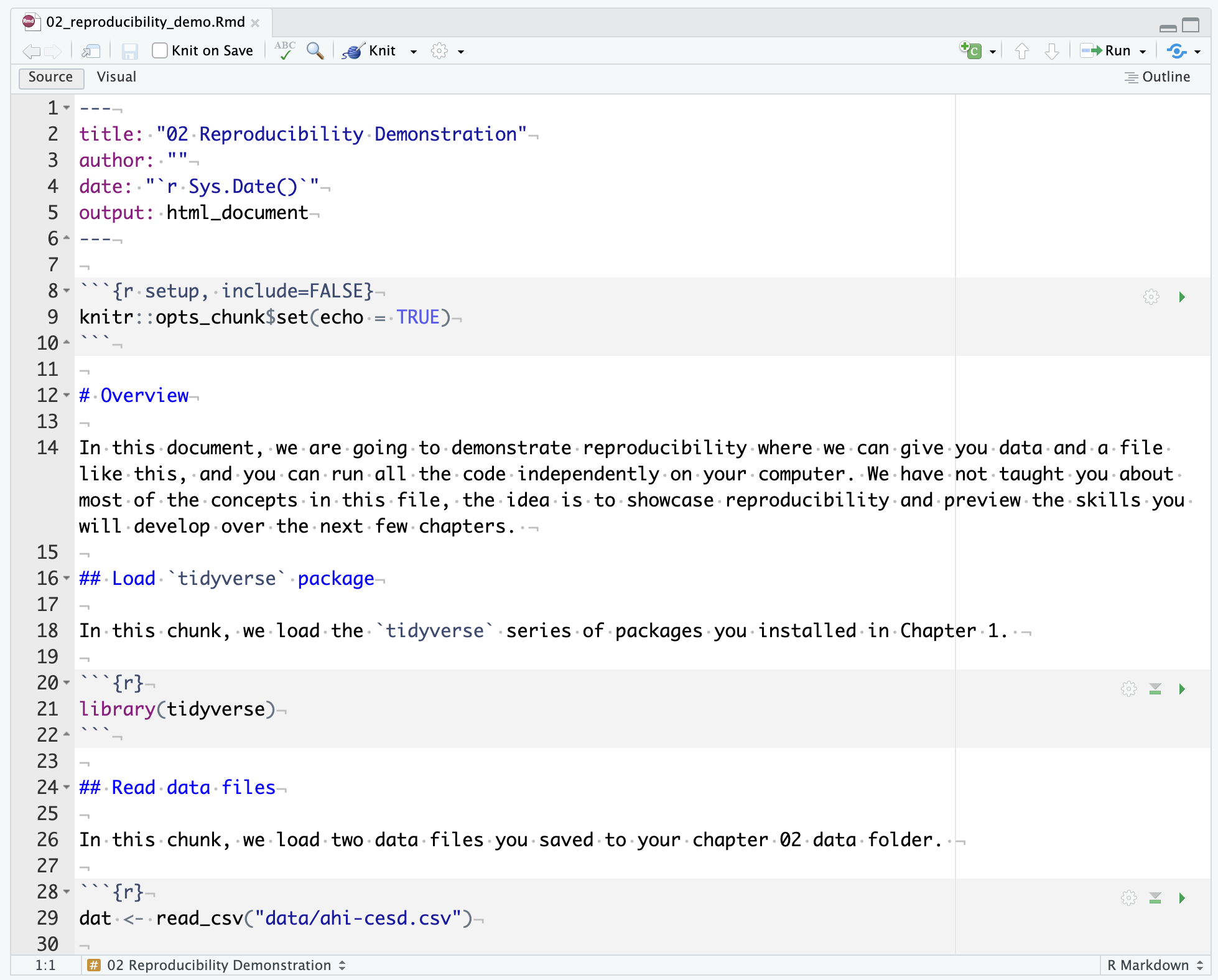
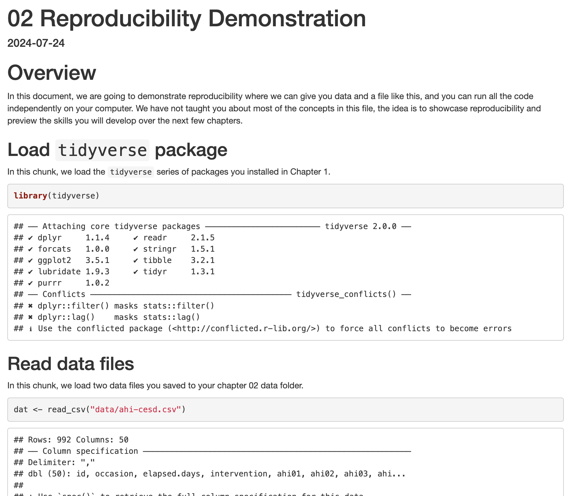
At the start of this chapter, we plugged the benefits of reproducible research as the ability to produce the same result for different people using the same software on different computers. We are going to end the chapter on a demonstration of this by giving you an R Markdown document and data. You should be able to click knit and see the results without editing anything. We do not expect you to understand the code included in it, we are previewing the skills you will develop over the next four chapters on visualisation and data wrangling.
2.3.1 Activity 9 - Knit the reproducibility demonstration document
Please follow these steps and you should be able to knit the document without editing anything. Make sure you are still in your Chapter_02_reproducible_docs folder. If you are coming back to this activity, remember to set your working directory by opening the .Rproj file.
If you are working on your own computer, make sure you installed the
tidyversepackage. Please refer to Chapter 1 - Activity 3 if you have not completed this step yet. If you are working on a university computer or the online server, you do not need to complete this step astidyversewill already be installed.Download the R Markdown document through the following link: 02_reproducibility_demo.Rmd. To download a file from this book, right click the link and select “save link as”, or just clicking the link will save the file to your Downloads. Save or copy the file to your
Chapter_02_reproducible_docsfolder.Download these two data files. Data file one: ahi-cesd.csv. Data file two: participant-info.csv. Right click the links and select “save link as”, or clicking the links will save the files to your Downloads. Make sure that both files are saved as “.csv”. Do not open them on your machine as often other software like Excel can change setting and ruin the files. Save or copy the file to your
data/folder withinChapter_02_reproducible_docs.
At this point, you should have “02_reproducibility_demo.Rmd” within your Chapter_02_reproducible_docs folder. You should have “ahi-cesd.csv” and “participant_info.csv” in the data/ folder within Chapter_02_reproducible_docs.
If you open “02_reproducibility_demo.Rmd” and followed all the steps above, you should be able to click knit. This will turn the R Markdown file into a knitted html file, showing some data wrangling, summary statistics, and two graphs (Figure 2.14). In the next chapter, you will learn how to write this code yourself, starting with creating graphs.
If you have any questions or problems about anything contained in this chapter, please remember you are always welcome to post on the course Teams channel, attend a GTA support session, or attend the office hours of one of the team.
2.4 Test yourself
To end the chapter, we have some knowledge check questions to test your understanding of the concepts we covered in the chapter. We then have some error mode tasks to see if you can find the solution to some common errors in the concepts we covered in this chapter.
2.4.1 Knowledge check
Question 1. One of the key first steps when we open RStudio is to:
Explain this answer
One of the most common issues we see where code does not work the first time is because people have forgotten to set the working directory. The working directory is the starting folder on your computer where you want to save any files, any output, or contains your data. R/RStudio needs to know where you want it to look, so you must either manually set your working directory, or open a .Rproj file.
Question 2. When using the default environment color settings for RStudio, what color would the background of a code chunk be in R Markdown?
Question 3. When using the default environment color settings for RStudio, what color would the background of normal text be in R Markdown?
Explain this answer
Assuming you have not changed any of the settings in RStudio, code chunks will tend to have a grey background and normal text will tend to have a white background. This is a good way to check that you have closed and opened code chunks correctly.
Explain this answer
Code chunks always take the same general format of three backticks followed by curly parentheses and a lower case r inside the parentheses ({r}). People often mistake these backticks for single quotes but that will not work. If you have set your code chunk correctly using backticks, the background color should change to grey from white
Explain this answer
Inline coding is an incredibly useful approach for merging text and code in a sentence outside of a code chunk. It can be really useful for when you want to add values from your code directly into your text. If you copy and paste values, you can easily create errors, so it’s useful to add inline code where possible.
2.4.2 Error mode
The following questions are designed to introduce you to making and fixing errors. For this topic, we focus on R Markdown and potential errors in using code blocks and inline code. Remember to keep a note of what kind of error messages you receive and how you fixed them, so you have a bank of solutions when you tackle errors independently.
Create and save a new R Markdown file by following the instructions in activity 3 and activity 4. You should have a blank R Markdown file below line 10. Below, we have several variations of a code chunk and inline code errors. Copy and paste them into your R Markdown file, click knit, and look at the error message you receive. See if you can fix the error and get it working before checking the answer.
Question 5. Copy the following text/code/code chunk into your R Markdown file and press knit. You should receive an error like Error while opening file. No such file or directory.
Explain the solution
Here, we wrote city <- "Glasgow" outside the code chunk. So, when we try and knit, it is not evaluated as code, and city does not exist as an object to be referenced in inline code. If you copy city <- "Glasgow" into the code chunk and press knit, it should work.
Question 6. Copy the following text/code/code chunk into your R Markdown file and press knit. You should receive an error like Error in parse(): ! attempt to use zero-length variable name which is not very helpful for diagnosing the problem.
Explain the solution
Here, we missed a final backtick in the code chunk. You might have noticed all the text had a grey background, so R Markdown thought everything was code. So, when it reached the inline code and text, it tried interpreting it as code and caused the error. If you add the final backtick to the code chunk, you should be able to click knit successfully.
Question 7. Copy the following text/code/code chunk into your R Markdown file and press knit. You should receive an error like Error while opening file. No such file or directory.
Explain the solution
Here, we tried using inline code before the code chunk. R Markdown runs the code from start to finish in a fresh environment. We tried referencing city in inline code, but R Markdown did not know it existed yet. To fix it, you need to move the inline code below the code chunk, so you create city before referencing it in inline code.
Question 8. Copy the following text/code/code chunk into your R Markdown file and press knit. This…works?
Explain the solution
Here, we have a sneaky kind of “error” where it knits, but it is not doing what we wanted it to do. In the inline code part, we only added code formatting city, we did not add the r to get R Markdown to interpret it as R code:
If you add the r after the first backtick, it should knit and add the city object in.
2.5 Words from this Chapter
Below, you will find a list of words that we used in this chapter that might be new to you in case you need to refer back to what they mean. The links in this table take you to the entry for the words in the PsyTeachR Glossary. Note that numerous members of the team wrote entries in the Glossary and as such the entries may use slightly different terminology from what we used in the chapter.
| term | definition |
|---|---|
| chunk | A section of code in an R Markdown file |
| html | Hyper-Text Markup Language: A system for semantically tagging structure and information on web pages. |
| inline-code | Directly inserting the result of code into the text of a .Rmd file. |
| knit | To create an HTML, PDF, or Word document from an R Markdown (Rmd) document |
| latex | A typesetting program needed to create PDF files from R Markdown documents. |
| markdown | A way to specify formatting, such as headers, paragraphs, lists, bolding, and links. |
| r-markdown | The R-specific version of markdown: a way to specify formatting, such as headers, paragraphs, lists, bolding, and links, as well as code blocks and inline code. |
| r-project | A project is simply a working directory designated with a .RProj file. When you open an R project, it automatically sets the working directory to the folder the project is located in. |
| reproducible-research | Research that documents all of the steps between raw data and results in a way that can be verified. |
| working-directory | The filepath where R is currently loading files from and saving files to. |
2.6 End of chapter
Well done on reaching the end of the second chapter! This was another long chapter as we had to cover a range of foundational skills to prepare you for learning more of the coding element in future chapters.
The next chapter builds on all the skills you have developed so far in R programming and creating reproducible documents to focus on something more tangible: data visualisation in R to create plots of your data.