5 Data wrangling 2: Filter and summarise
One of the key aspects in a researcher’s toolbox is the knowledge and skill to work with data regardless of how it comes to you. When you run a study, you might get lots of different data types in various different files. For instance, some experimental software creates a new file for every participant, and each participant’s file might contain columns and rows of different data types, only some of which are important. Being able to wrangle that data, manipulate it into different layouts, extract the parts you need, and summarise it, is one of the most important skills we will help you learn throughout this book.
In the last chapter, we introduced you to several one-table functions from
In this chapter, we are going to continue developing our understanding of data, and build on the knowledge and skills you have developed so far. We start with a recap of data wrangling functions from Chapter 4 and ask you to apply them to a new data set. Feel free through to refer back to Chapter 4 for help - this is not a test - but try and complete the activities independently to judge how well you can transfer your skills to a new scenario. We then introduce you to new data wrangling functions to filter and summarise.
Chapter Intended Learning Outcomes (ILOs)
By the end of this chapter, you will be able to:
Apply your data wrangling skills to a new unseen data set.
Filter observations to retain a subset of your data, such as keeping only postgraduate students.
Summarise your data to calculate summary statistics, either across all of your observations, or by subsetting across one or more additional variables.
5.1 Chapter preparation
5.1.1 Introduction to the data set
For this chapter, we are using open data from Witt et al. (2018). The abstract of their article is:
Can one’s ability to perform an action, such as hitting a softball, influence one’s perception? According to the action-specific account, perception of spatial layout is influenced by the perceiver’s abilities to perform an intended action. Alternative accounts posit that purported effects are instead due to nonperceptual processes, such as response bias. Despite much confirmatory research on both sides of the debate, researchers who promote a response-bias account have never used the Pong task, which has yielded one of the most robust action-specific effects. Conversely, researchers who promote a perceptual account have rarely used the opposition’s preferred test for response bias, namely, the postexperiment survey. The current experiments rectified this. We found that even for people naive to the experiment’s hypothesis, the ability to block a moving ball affected the ball’s perceived speed. Moreover, when participants were explicitly told the hypothesis and instructed to resist the influence of their ability to block the ball, their ability still affected their perception of the ball’s speed.
To summarise, their research question was: does your ability to perform an action influence your perception? For instance, does your ability to hit a tennis ball influence how fast you perceive the ball to be moving? Or to phrase another way, do expert tennis players perceive the ball moving slower than novice tennis players?
This experiment does not use tennis players, instead they used the Pong task like the classic retro arcade game. Participants aimed to block moving balls with various sizes of paddles. Participants tend to estimate the balls as moving faster when they have to block it with a smaller paddle as opposed to when they have a bigger paddle. In this chapter, we will wrangle their data to reinforce skills from Chapter 4, and add more
5.1.2 Organising your files and project for the chapter
Before we can get started, you need to organise your files and project for the chapter, so your working directory is in order.
In your folder for research methods and the book
ResearchMethods1_2/Quant_Fundamentals, you should have a folder from chapter 4 calledChapter_04_06_datawranglingwhere you created an R Project.Create a new R Markdown document and give it a sensible title describing the chapter, such as
05 Data Wrangling 2. Delete everything below line 10 so you have a blank file to work with and save the file in yourChapter_04_06_datawranglingfolder.We are working with a new data set, so please save the following data file: witt_2018.csv. Right click the link and select “save link as”, or clicking the link will save the files to your Downloads. Make sure that you save the file as “.csv”. Save or copy the file to your
data/folder withinChapter_04_06_datawrangling.
You are now ready to start working on the chapter!
5.2 Select, arrange, and mutate recap
Before we introduce you to new functions, we will recap data wrangling functions from Chapter 4 to select, arrange, and mutate. Following along is one thing but being able to transfer your understanding to a new data set is a key sign of your skill development. Feel free to use Chapter 4 to help you, but try and complete the recap activities independently before checking the solutions. This will help prepare you as we move from the chapters, to the data analysis journeys, to the assessments, and to your future career.
5.2.1 Activity 1 - Load tidyverse and read the data file
As the first activity, try and test yourself by loading
5.2.2 Activity 2 - Explore pong_data
Remember the first critical step when you come across any new data is exploring to see how many columns you are working with, how many rows/observations there are, and what the values look like. For example, you can click on pong_data in the environment and scroll around it as a tab. You can also get a preview of your data by using the glimpse() function.
Rows: 4,608
Columns: 8
$ Participant     <dbl> 1, 1, 1, 1, 1, 1, 1, 1, 1, 1, 1, 1, 1, 1, 1, 1, 1, 1, …
$ JudgedSpeed     <dbl> 1, 0, 1, 0, 1, 0, 1, 0, 0, 0, 1, 1, 0, 1, 0, 1, 0, 1, …
$ PaddleLength    <dbl> 50, 250, 50, 250, 250, 50, 250, 50, 250, 50, 50, 250, …
$ BallSpeed       <dbl> 5, 3, 4, 3, 7, 5, 6, 2, 4, 4, 7, 7, 3, 6, 5, 7, 2, 5, …
$ TrialNumber     <dbl> 1, 2, 3, 4, 5, 6, 7, 8, 9, 10, 11, 12, 13, 14, 15, 16,…
$ BackgroundColor <chr> "red", "blue", "red", "red", "blue", "blue", "red", "r…
$ HitOrMiss       <dbl> 0, 1, 0, 1, 1, 1, 1, 1, 1, 1, 0, 1, 1, 1, 1, 0, 1, 1, …
$ BlockNumber     <dbl> 1, 1, 1, 1, 1, 1, 1, 1, 1, 1, 1, 1, 1, 1, 1, 1, 1, 1, …
If you look at that table, you can see there are 8 columns and 4608 rows. Seven of the column names are <dbl>, short for double, and one is <chr>, short for character. We will need to keep the data types in mind as we wrangle the data.
5.2.3 Data types in R
We try and balance developing your data skills in a practical way while slowly introducing some of the underlying technical points. In the last chapter, we warned about honoring data types so R knew how to handle numbers/doubles vs factors. Now we have explored a few data sets, it is time to clarify some key differences between data types in R.
We often store data in two-dimensional tables, either called data frames, tables, or tibbles. There are other ways of storing data that you will discover in time but in this book, we will be using data frame or tibbles (a special type of data frame in the tidyverse). A data frame is really just a table of data with columns and rows of information. Within the cells of the data frame - a cell being where a row and a column meet - you get different types of data, including double, integer, character and factor. To summarise:
| Type of Data | Description |
|---|---|
| Double | Numbers that can take decimals |
| Integer | Numbers that cannot take decimals |
| Character | Tends to contain letters or be words |
| Factor | Nominal (categorical). Can be words or numbers (e.g., animal or human, 1 or 2) |
Double and integer can both be referred to as numeric data, and you will see this word from time to time. For clarity, we will use double as a term for any number that can take a decimal (e.g. 3.14) and integer as a term for any whole number (no decimal, e.g. 3).
Somewhat confusingly, double data might not have decimal places in it. For instance, the value of 1 could be double as well as integer. However, the value of 1.1 could only be double and never integer. Integers cannot have decimal places. The more you work with data the more this will make sense, but it highlights the importance of looking at your data and checking what type it is as the type determines what you can do with the data.
In pong_data, each row (observation) represents one trial per participant and there are 288 trials for each of the 16 participants. Most of the data is a double (i.e., numbers) and one column is a character (i.e., text). The columns (variables) we have in the data set are:
| Variable | Type | Description |
|---|---|---|
| Participant | double | participant number |
| JudgedSpeed | double | speed judgement (1 = fast, 0 = slow) |
| PaddleLength | double | paddle length (pixels) |
| BallSpeed | double | ball speed (2 pixels/4ms) |
| TrialNumber | double | trial number |
| BackgroundColor | character | background display colour |
| HitOrMiss | double | hit ball = 1, missed ball = 0 |
| BlockNumber | double | block number (out of 12 blocks) |
5.2.4 Activity 3 - select() a range of columns
Either by inclusion (stating all the variables you want to keep) or exclusion (stating all the variables you want to drop), create a new object named select_dat and select the following columns from pong_data:
ParticipantPaddleLengthTrialNumberBackgroundColorHitOrMiss
5.2.5 Activity 4 - Reorder the variables using select()
We can also use select() to reorder your columns, as the new data object will display the variables in the order that you entered them.
Use select() to keep only the columns Participant, JudgedSpeed, BallSpeed, TrialNumber, and HitOrMiss from pong_data but this time, display them in ascending alphabetical order. Save this tibble in a new object named reorder_dat.
5.2.6 Activity 5 - Reorder observations using arrange()
Reorder observations in the data using the following two variables: HitOrMiss (putting hits (1) first) and JudgedSpeed (putting fast judgement (1) first). Store this in an object named arrange_dat.
Now try and answer the following questions about the data.
What is the trial number (
TrialNumber) in the 1st row?What is the background colour (
BackgroundColor) in the 10th row?
You needed to include desc() to change it from running smallest-to-largest to largest-to-smallest as the values are 0 and 1. You should have the following in a code chunk:
5.2.7 Activity 6 - Modifying or creating variables using mutate()
Some of these values could be a little easier to understand. They are represented in the data by 0s and 1s, but it might not be immediately obvious what they mean.
Create a new variable called JudgedSpeedLabel by mutating the original pong_data object. Change the values in JudgedSpeed using the following labels:
0 = Slow
1 = Fast
5.3 Removing or retaining observations using filter()
Now we have revisited key data wrangling functions from Chapter 4 to select, arrange, and mutate, it is time to add some new functions from
Using select, we could remove columns, but there are many situations where you want to include or exclude certain observations/rows. The function filter() will possibly be one of your most used for data wrangling. For example, imagine you want to only analyse participants who provided informed consent and exclude participants who did not. Similarly, you might want to focus your analyses only on participants who are under the age of 21.
5.3.1 Activity 7 - Filter using one criterion
We will jump straight into an example. Imagine that you realised you made a mistake creating your experiment and all your trial numbers are wrong. The first trial (trial number 1) was a practice, so you should exclude it and your experiment actually started on trial 2.
To break down the code:
We create a new object called
pong_data_filterby applying the filter function topong_data.We add the Boolean expression
TrialNumber > 1to keep all responses higher than 1 (i.e., 2 or higher).
The filter() function uses our old friends the Boolean expressions we introduced you to in Chapter 4. You can add one or more logical expressions to filter observations. The function retains observations when they are evaluated to TRUE and ignores observations when they are evaluated to FALSE. Remember, when you are working out how to express your ideas in code, test them out. For example, we can see what the expression would do to different trial numbers:
1 is not larger than 1, so it’s evaluated to FALSE and would be ignored. 2 is larger than 2, so it’s evaluated to TRUE and would be retained. Explore the two data sets pong_data and pong_data_filter and the number of rows they have to see the effects of applying the function.
As a reminder from Chapter 4, the most common Boolean expressions are:
| Operator | Name | is TRUE if and only if |
|---|---|---|
| A < B | less than | A is less than B |
| A <= B | less than or equal | A is less than or equal to B |
| A > B | greater than | A is greater than B |
| A >= B | greater than or equal | A is greater than or equal to B |
| A == B | equivalence | A exactly equals B |
| A != B | not equal | A does not exactly equal B |
| A %in% B | in | A is an element of vector B |
Using the filter() example and the table above, imagine we wanted to only keep trials where participants judged the speed to be “Fast”. Use the pong_data_filter after removing trial number 1 and assign it to a new object pong_data_fast. You could use the JudgedSpeed or JudgedSpeedLabel variable to do this.
For a hint, you want to keep responses when they are equivalent to “Fast” or 1 depending on the variable you use.
You were looking for the equivalence Boolean operator (==) to retain responses which were equal to “Fast” or 1. If you used JudgedSpeedLabel, you should have:
If you used JudgedSpeed, you should have:
Note we use a double equals == and not a single equals = for the Boolean operator. We also must honour the data type for the expression we set.
5.3.2 Activity 8 - Filter using two or more criteria
You explored using one criterion to filter out or retain observations/rows, but you can make the expressions arbitrarily more complicated by adding two or more criteria to evaluate against. Just note the more criteria you add, the more selective you are being. You are probably going to be excluding more and more observations, so think about what you want to achieve.
Focusing on one variable, you can specify multiple values to compare against. For example, you might want to only keep responses which had a ball speed of 2 or 4:
To break down the code:
We create a new object called
pong_data_BallSpeedby applying the filter function topong_data_filter.We add the Boolean expression
BallSpeed == 2, the vertical line symbol (|), then a second expressionBallSpeed == 4. The vertical line symbol (|) means “or”, so our expression is retainBallSpeedresponses which equal 2 OR 4, and ignore all the others.
For two values, this is pretty straightforward, but it could get out of hand when you have four or five values to evaluate against. There is a super handy shortcut from the Boolean expressions table for “in” which we can apply if we wanted to keep ball speeds of 2, 4, 5, and 7:
You can read the expression here as: for each observation/row, check whether the value of BallSpeed is in the vector of numbers 2, 4, 5, 7. Remember filter() works by whether the expression is evaluted to TRUE or FALSE, so you can see how it works by testing some numbers:
1 is not present in c(2, 4, 5, 7), so it is evaluated to FALSE and would be ignored. 2 is presented in c(2, 4, 5, 7), so it is evaluated to TRUE and would be retained.
You can also add two or more expressions including multiple variables by adding them to the function separated by commas. For example, imagine we wanted to retain observations/rows which had a “Fast” speed judgement with ball speeds of 2, 4, 5, and 7:
In the first expression, we only want to keep observations/rows which have a JudgedSpeedLabel of “Fast”. In the second expression, we only want to keep observations/rows which have a BallSpeed of 2, 4, 5, or 7. In other words, retain “Fast” observations AND those with a ball speed of 2, 4, 5, or 7. Adding more expressions makes your criteria more selective as rows must pass both conditions to be retained in the data.
Using the examples above, imagine we wanted to only keep trials where:
The
PaddleLengthis 50.The
BackgroundColoris red.The
HitOrMissis 1.
Use the pong_data_filter object and assign it to a new object pong_data_three_criteria.
5.4 Counting observations using count()
As we work from wrangling data towards analysing your data to produce numerical summaries, we can start introducing different ways of summarising your data set.
In it’s simplest sense, we can look at different ways of counting your observations. Often, it is helpful to know how many observations you have, either in total, or broken down by groups. This can help you spot if something has gone wrong in a calculation, e.g., if you have done something with the code and your mean or median is only being calculated using a subset of the values you intended. Alternatively, it can be useful for reporting descriptive statistics, such as how many participants were in your study or how many people were in each group.
5.4.1 Activity 9 - Counting observations
To count observations, you have the function count(). Without any additional arguments, you can use the function to report how many observations are in your data set:
This corresponds nicely with the number of observations you can see in the data environment window and from when we have used glimpse() for a summary of the object.
You can then add one or more variables to the function to count the number of observations within each variable and across the combination of variables when you supply two or more. For example, we could count the number of observations within BackgroundColor:
And it would give the answer of:
| BackgroundColor | n |
|---|---|
| blue | 2304 |
| red | 2304 |
We can see there are an equal number of blue and red backgrounds across all the observations.
One way of sense checking your data and making sure there is not a sneaky error is checking how many observations there are per unique participant and ensuring that matches up with what you understand about the study.
Use the count() function on the pong_data_filter object to answer the following questions about the data:
How many observations do we have for each unique
Participantin the data?HitOrMisscodes for whether theParticipanthit or missed the ball in the trial. If you count the number ofHitOrMissperParticipant, participant number 3 made hits and misses.
To answer question 1, we only need to add Participant as an argument after the data pong_data_filter.
To answer question 2, we need both Participant and HitOrMiss as arguments after the data pong_data_filter, as we want the number of hits and misses per participant.
5.5 Summarising data using summarise() and group_by()
Counting data is useful, but it might not be the only way of summarising data that you want. A more flexible function is summarise() which you can use to calculate summary statistics across your whole data frame, or grouped by additional variables.
5.5.1 Activity 10 - Summarising all the observations
To start with something familiar, we can use summarise() to count observations. The function works in a similar format to mutate() where you enter a variable name and tell R what function you want applying to the data frame or variable. For example, we can use the n() function to calculate the number of observations in pong_data_filter:
To break down the code:
We create a new object
N_observationsby applying thesummarise()function topong_data_filter.We create a new variable name called
N_observations, add an equals for what that new variable represents, and add our desired functionn(). You do not need to add any further arguments, it calculates the number of observations in the object you give it.
This creates a new object as a data frame with 1 observation and 1 column to produce a single number:
| N_observations |
|---|
| 4592 |
Reassuringly, this is exactly the same as we received for count(). If you only want the number of observations, then count() will be more efficient. However, if you want to produce the number of observations in addition to other summary statistics, then summarise() is going to be more useful.
To demonstrate the flexibility of summarise(), we can add another summary statistic for the mean hit rate. When binary outcomes like a hit or a miss are coded as 0 and 1, taking the mean provides the proportion of hits (or whatever is coded as 1).
| N_observations | hit_proportion |
|---|---|
| 4592 | 0.6879355 |
In this example, we have not saved the summarise() output to a new object, just printed it’s result. We can see we get the number of observations as before, but we also get the mean value for the hit rate. The proportion of hits across all observations was 0.688 or 68.8%.
When you use the mean() function, you might find the result is NA. This is likely due to the presence of an NA or missing value in your variable. NAs are contagious as if you try and calculate the mean of a set of numbers containing one or more NA values, the overall mean will also be an NA.
So, the mean() function has an additional argument na.rm = TRUE which tells R what to do if there are missing values. The job of na.rm is to say whether to remove (rm) the NAs (na.rm = TRUE) or not (na.rm = FALSE).
This data set has no missing values but we showed you how to use it here so you can try to remember it exists in future. You do not need to use it all the time and you should think carefully about whether you should ignore NAs, but the option is there if you need it.
Using what you learnt above, apply the summarise() function to calculate the mean value of JudgedSpeed using the pong_data_filter object and fill in the blanks below. Remember, calculating the mean of a binary outcome of 0s and 1s tells you the proportion, so the mean here would be the proportion of responses judged to be fast.
Rounded to 3 decimal places, the mean proportion of fast responses is or rounded to 1 decimal place %.
You only needed to add one argument to calculate the mean of the JudgedSpeed variable. We called the new variable fast_proportion, but this was not important for the answer. Just make sure you call your variables something sensible, so you could understand what it means later.
5.5.2 Activity 11 - Grouping your summary statistics
Summarising your whole data set is great, but there will often be times you want separate summary statistics for different groups in your data. The group_by() function takes an existing data frame or tibble and creates a grouped data frame. As a data frame, this does not look much different, but it adds a kind of hidden property which functions like summarise() detects and uses.
As an example, let us see how the summary statistics compare between each level of judged speed. For the initial step, we need to apply the group_by() function:
To break down the code:
We create a new object
pong_data_groupedby applying thegroup_by()function topong_data_filter.We add one or more variables we want to group any summary statistics by. In this case, we group by
JudgedSpeedLabelso we will get separate values for fast and slow.
If you open pong_data_grouped as a tab, it does not look any different. Remember, group_by() adds a kind of hidden property. To check this, we can run the str() function on the data object which will show us the structure of an object:
gropd_df [4,592 × 9] (S3: grouped_df/tbl_df/tbl/data.frame)
 $ Participant     : num [1:4592] 1 1 1 1 1 1 1 1 1 1 ...
 $ JudgedSpeed     : num [1:4592] 0 1 0 1 0 1 0 0 0 1 ...
 $ PaddleLength    : num [1:4592] 250 50 250 250 50 250 50 250 50 50 ...
 $ BallSpeed       : num [1:4592] 3 4 3 7 5 6 2 4 4 7 ...
 $ TrialNumber     : num [1:4592] 2 3 4 5 6 7 8 9 10 11 ...
 $ BackgroundColor : chr [1:4592] "blue" "red" "red" "blue" ...
 $ HitOrMiss       : num [1:4592] 1 0 1 1 1 1 1 1 1 0 ...
 $ BlockNumber     : num [1:4592] 1 1 1 1 1 1 1 1 1 1 ...
 $ JudgedSpeedLabel: chr [1:4592] "Slow" "Fast" "Slow" "Fast" ...
 - attr(*, "groups")= tibble [2 × 2] (S3: tbl_df/tbl/data.frame)
  ..$ JudgedSpeedLabel: chr [1:2] "Fast" "Slow"
  ..$ .rows           : list<int> [1:2]
  .. ..$ : int [1:2512] 2 4 6 10 11 13 15 17 19 22 ...
  .. ..$ : int [1:2080] 1 3 5 7 8 9 12 14 16 18 ...
  .. ..@ ptype: int(0)
  ..- attr(*, ".drop")= logi TRUE
The two key elements here are in the first line (gropd_df [4,592 × 9] (S3: grouped_df/tbl_df/tbl/data.frame)) and below the variables (- attr(*, "groups")... ..$ JudgedSpeedLabel: chr [1:2] "Fast" "Slow"). The first line confirms we now have a grouped data frame and the two lines below the variables show the values we group by.
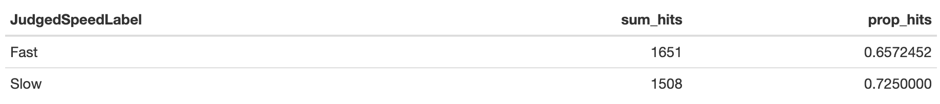
The next step is applying the summarise() function as before. Here, we will calculate the total and mean number of hits by whether the participants judged the speed to be fast or slow:
Calling the object shows we now get two rows per summary statistic:
Although there were more hits in the fast judged speed, the proportion of hits to misses was lower. Participants hit .657 (65.7%) of trials they judged to be fast but .725 (72.5%) of trials they judged to be slow.
Using what you learnt above, apply the group_by() and summarise() functions to calculate the sum and mean value of HitOrMiss depending on whether BackgroundColor was blue or red. In your group_by() object, make sure you use the pong_data_filter object. After writing the code and checking the new object, answer the following questions:
Rounded to 2 decimal places, the mean proportion of hits to the blue background was or rounded to 0 decimal places %.
Rounded to 3 decimal places, the mean proportion of hits to the red background was or rounded to 1 decimal place %.
There are two steps here to follow the previous example. The main difference is using BackgroundColor in group_by(), and then the summarise() element is largely the same.
After we introduced you to R Markdown to create reproducible documents in Chapter 2, we are going to add a tip in every chapter to demonstrate extra functionality.
R Markdown is great for embedding plots and statistics in reproducible documents, but tables can be a little tricky. If you only call objects like hits_by_background, the output does not look super professional and it is not consistent with APA formatting guidelines.
There are a few options available to you. One of the packages that helps create R Markdown - kable() which can create tables with no further arguments, but you will need to edit the object to make sure it has headers and labels consistent with APA. The following code creates a simple table if you have
You will need to knit your document to see what it looks like, but it should look similar to Figure 5.1. The row labels are fine, but you would need to tidy up the headers and round prop_hits to three decimals (see the function round()).
See The R Markdown Cookbook for a guide on creating tables using kable().
Alternatively, there is a package called
5.5.3 Ungrouping data
For a final word of warning, there is an additional function which removes a group from a data frame. For example, if you wanted to use objects like pong_data_grouped for additional wrangling, visualisation, or analysis, it can create problems if you leave the group property. If you only use these objects to create summary tables like hits_by_judgedspeed, then there is no issue.
It is good practice to ungroup the data before performing another function using the ungroup() function:
If you run str(pong_data_grouped) again, you will see we removed the grouping property. Remember, you only need to apply this if you are using the object in further steps. We will demonstrate in the next chapter how you can add this in a more streamlined way.
5.6 Test yourself
To end the chapter, we have some knowledge check questions to test your understanding of the concepts we covered in the chapter. We then have some error mode tasks to see if you can find the solution to some common errors in the concepts we covered in this chapter.
5.6.1 Knowledge check
Question 1. What type of data would these most likely be:
Male =
7.15 =
137 =
There are several different types of data as well as different levels of measurement and it takes a while to recognise the nuanced differences. It is important to try to remember which is which because you can only do certain types of analyses on certain types of data and certain types of measurements. For instance, you cannot take the average of characters or categorical data. Likewise, you can do any maths on double data, just like you can on interval and ratio data. Integer data is funny in that sometimes it is ordinal and sometimes it is interval, sometimes you should take the median, sometimes you should take the mean. The main point is to always know what type of data you are using and to think about what you can and cannot do with them.
Note: in the last answer, 137 could also be double as it is not clear if it could take a decimal or not.
5.6.2 Error mode
The following questions are designed to introduce you to making and fixing errors. For this topic, we focus on data wrangling using the functions filter(), count(), and group_by() and summarise(). Remember to keep a note of what kind of error messages you receive and how you fixed them, so you have a bank of solutions when you tackle errors independently.
Create and save a new R Markdown file for these activities. Delete the example code, so your file is blank from line 10. Create a new code chunk to load tidyverse and the data file:
Below, we have several variations of a code chunk error or misspecification. Copy and paste them into your R Markdown file below the code chunk to load tidyverse and the data. Once you have copied the activities, click knit and look at the error message you receive. See if you can fix the error and get it working before checking the answer.
Question 6. Copy the following code chunk into your R Markdown file and press knit. We want to filter data to only include a paddle length of 50. You should receive the error starting with Error in "filter()" ! We detected a named input.
```{r}
# filter pong_data to retain PaddleLength of 50
pong_data_filter <- filter(pong_data,
                           PaddleLength = 50)
```In the code, we use a single equals sign (=) rather than the Boolean operator a double equals sign (==). With a single equals, R is interpreting this as “PaddleLength is equal to 50” like you were saving an object or setting an argument. The error message below line two tries to help and suggests you might need to include == instead.
Question 7. Copy the following code chunk into your R Markdown file and press knit. We want to count the number of trials per block (BlockNumber). This…works, but if you look at the output, have we counted the number of trials?
```{r}
# Count block numbers from pong_data
count_blocknumbers <- summarise(pong_data,
                                N_blocks = sum(BlockNumber))
```Question 8. Copy the following code chunk into your R Markdown file and press knit. Here, we want the proportion of fast judgements per paddle length by taking the mean of JudgedSpeed. This code… works, but do we have a proportion of fast judgements per paddle length?
```{r}
# Mean judged speed for the proportion of fast judgements
hits_by_background <- summarise(pong_data,
                                prop_fast = mean(JudgedSpeed))
```We wanted the mean proportion of fast judgements, but we forgot to add a group by! We only got one value, so we need to add an initial step to group the responses by PaddleLength first, before we then calculate the mean proportion.
5.7 Words from this Chapter
Below you will find a list of words that were used in this chapter that might be new to you in case it helps to have somewhere to refer back to what they mean. The links in this table take you to the entry for the words in the PsyTeachR Glossary. Note that the Glossary is written by numerous members of the team and as such may use slightly different terminology from that shown in the chapter.
| term | definition |
|---|---|
| character | A data type representing strings of text. |
| count() | Count the observations in your data set, or the number of observations in one or more variables. |
| data-frame | A container data type for storing tabular data. |
| double | A data type representing a real decimal number |
| factor | A data type where a specific set of values are stored with labels; An explanatory variable manipulated by the experimenter |
| filter() | The ability to subset a data frame to keep all observations/rows that satisfy one or more conditions. |
| function | A named section of code that can be reused. |
| group_by() | Take an existing data frame or tibble and convert it to a grouped data frame. |
| integer | A data type representing whole numbers. |
| numeric | A data type representing a real decimal number or integer. |
| summarise() | Creates a new data frame to summarise all the observations you provide. You can also group by an additional variable to create separate summary statistics. |
| tibble | A container for tabular data with some different properties to a data frame |
| ungroup() | Remove a grouping property from a grouped data frame or tibble. |
5.8 End of chapter
Brilliant work again! You have another handful of functions added to your data wrangling toolkit and we are almost ready to tackle more advanced plotting techniques and inferential statistics.
In the next chapter, we finish the key data wrangling functions. For example, showing you how you can pipe together multiple functions to streamline your code. We will also demonstrate how to pivot your data wider from long form where there are multiple observations per participant to wide form where there is one row per participant, and vice versa.