21  Reporting Power Analyses

In this research skills chapter, we explore reporting power analyses which normally goes in the method, but it does not quite align with the schedule for how quickly we cover report writing and inferential statistics. A power analysis is one strategy to justify how many participants you require for your study, and you would typically include it in the participants or data analysis sub-section of the method. We wanted to make sure we cover reporting power for anyone who wants to go above and beyond in the stage one group report.

21.1 Recommended resources for statistical power

In semester 1, the concept of statistical power and how it applies to specific statistical tests are spread across materials and several weeks of lectures:

• Lecture week 5 - Hypothesis testing.

• Lectures week 7-9 - Inferential statistics for correlations, t-tests, and regression.

• Chapter 10 of the PsyTeachR book Fundamentals of Quantitative Analysis outlines how to perform power analysis in R for different statistical tests.

• Bartlett and Charles (2022) provide a beginner’s tutorial to power analysis. Part 1 outlines the concept of statistical power and part 2 discusses justifying the inputs you use in power analysis. Ignore part 3 as you will be using R instead of jamovi.

21.2 Statistical power recap

In null hypothesis significance testing (NHST), we can put a limit on two types of error. Type I errors (false positives) are when we reject the null hypothesis and conclude a test was statistically significant, when really the null hypothesis is true. Type II errors (false negatives) are when we retain the null hypothesis and conclude a test was non-significant, when really the null hypothesis is false.

Statistical power is related to the second type of error (type II). The definition of power is the long run probability of your study design correctly rejecting the null hypothesis when there is a true effect to be found. In short, “if an effect exists, how likely am I to detect it”? If a study has high statistical power, you would reliably detect a given effect size. If a study has low statistical power, you would not reliably detect a given effect size.

In null hypothesis significance testing, there are four key concepts:

• Alpha: The predetermined cut-off in your design at which you reject the null hypothesis (normally set at $\alpha$ = .05). This is your false positive error rate to limit the number of type I errors you would be willing to make.

• Power: The ability of a design to find an effect based on 1 - $\beta$, where beta is normally set at .20 or .10, producing power = .80 or .90. Beta is the false negative error rate to limit the number of type II errors you would be willing to make.

• Effect size: A number that expresses the magnitude of the phenomenon related to your research question. This will typically be Cohen’s d for the standardised mean difference in t-tests or the correlation coefficient r.

• Sample size: The number of participants or observations in your study.

Conveniently, there is an interaction between the four key concepts of Alpha, Power, Effect Size, and Sample Size (APES). If you state three, you can calculate the fourth. Assuming you use the field standards of $\alpha$ = .05 and power = .80, choosing the final input of sample size or effect size produces one of two informative types of power analysis:

1. A priori power analysis: You solve power analysis for the number of participants you need for a given value of $\alpha$, power, and effect size.

2. Sensitivity power analysis: You solve power analysis for the effect size you can detect for a given value of $\alpha$, power, and sample size.

For an example, Mehr et al. (2016, pg. 487) report the following a priori power analysis in their study on the effect of melody on infants:

“Statistical power. The target sample size of 32 was determined before the experiment began, to ensure adequate power to detect a positive selective-attention effect. A similar experiment testing effects of language rather than music (Kinzler et al., 2007) obtained an effect size (d) of 0.54, and a sample of 32 had .84 power to detect an effect of this magnitude.”

We can reproduce their power analysis using the pwr package for a paired samples t-test (if you have not got to Chapter 10 in data skills yet, do not worry if this looks unfamiliar):

pwr.t.test(d = 0.54,
           sig.level = .05,
           power = .84,
           type = "paired",
           alternative = "two.sided")

     Paired t test power calculation 

              n = 31.91057
              d = 0.54
      sig.level = 0.05
          power = 0.84
    alternative = two.sided

NOTE: n is number of *pairs*

Since we left the argument n blank, we receive that as the output of our a priori power analysis. We need 31.91 participants, but we always round up to a whole number of participants to avoid underestimating, so we would need 32 participants. The power analysis in Mehr et al. provides one example, but it is not perfect. There are some inputs they do not explicitly specify, so we will return to this example in reporting your power analysis below.

For your stage one report (and looking forward to your dissertation), you could report an a priori power analysis to inform how many participants you would need to detect your smallest effect size of interest. Power analysis and pre-registration is most informative in the design phase of research, so you would typically perform a power analysis to inform how many participants you try and recruit.

Just keep in mind: for the assignment in RM1 you have no control over the final sample size as we collected data for you. This means there might be a difference in your planned sample size from the a priori power analysis and the final sample size you work with. Therefore, we have a section on sensitivity power analysis to consider potential differences in your planned vs final sample size.

21.3 Choosing a smallest effect size of interest

For an a priori power analysis, you need to enter an effect size. The term we use for this is the smallest effect size of interest. It is rare you would know precisely what effect size you were looking for - as you would not need the study if you understood the topic that well. This means your smallest effect size of interest represents the threshold for what effect sizes you want your study sensitive enough to detect. Power exists along a curve, so holding the sample size and all other inputs constant, you would be less likely to detect smaller effects, but more likely to detect effects larger than your smallest effect of interest.

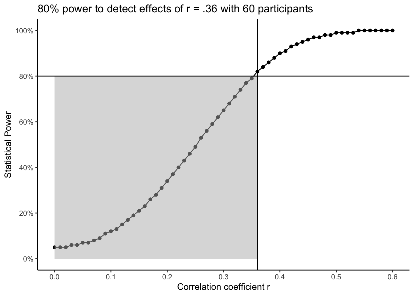
The following plot is a power curve showing the relationship between the correlation coefficient r as the effect size and statistical power for a given sample size. Assuming our power analysis suggested we need to collect 60 participants, we would have 80% power to detect effects of r = .36. The smallest effect size of interest is where the two lines meet for your desired level of power (here 80%). As you move down the curve highlighted by the grey region, you would be less likely to detect effects smaller than your smallest effect size of interest. As you move up the curve, you would be more likely to detect effects larger than your smallest effect size of interest. In short, and assuming you want to keep power at 80% or higher, then you would be looking for effect sizes at, or greater than, your smallest effect size of interest.

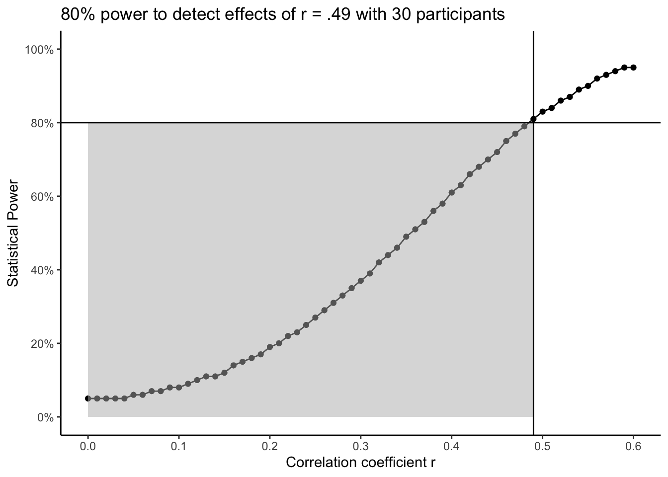
To demonstrate what this looks like for a larger smallest effect size of interest, if your power analysis suggested we need 30 participants, we would have 80% power to detect effects of r = .49. The smallest effect size of interest is again represented by where the two lines meet. Since we only wanted our design to be sensitive to larger effects, there is a larger grey region to highlight the effects we would be less likely to detect. As you move down the curve, you would be less likely to detect effects smaller than r = .49. As you move up the curve, you would be more likely to detect effects larger than r = .49. In short, you would be still be looking for effect sizes at, or greater than, your smallest effect size of interest, but that threshold shifts to exclude a larger region of smaller effects.

Assuming you use the field standards of $\alpha$ = .05 and power = .80, this leaves the smallest effect size of interest as the main decision you must make. Choosing an effect size is the hardest part of power analysis, but there is no one correct answer, only a difference between justified and unjustified. In your power analysis, we care more about your justification for your choice of effect size rather than the value itself.

You could always aim for a tiny effect size but in a real study you are trying to compromise between an informative study and the resources (time / money) you have available. You could always aim for a large effect size, but you might miss potentially informative smaller effects. This means you must choose your smallest effect size of interest based on your understanding of the topic area and consider what effects you would not want to miss out on.

There are different strategies for choosing a smallest effect size of interest (see Lakens, 2022 for a full discussion):

• Individual published studies: What effect sizes do similar studies to yours report?

• Meta-analyses: What is the average effect size across several studies on a topic?

• Effect size distributions: For a given topic, what is the distribution of effect sizes for what is considered small, medium, and large?

21.4 Reporting your power analysis

If you do report a power analysis, think about what information would allow the reader to reproduce your power analysis and understand your justification behind each input. Bakker et al. (2020) reviewed power analyses reported in pre-registrations and review boards and highlighted the most common omissions. From a sample of 210 studies, the most common omissions (% is the percentage of studies missing the information) in the features of a power analysis were:

• Sidedness of the test (78%)

• Justification for effect size (45%)

• Type of effect size (30%)

• Alpha value (29%)

• Value of effect size (15%)

• Power / beta value (15%)

• Sample size (8%)

Bakker et al. observed that the most common omission was whether researchers assumed a one- or two-tailed test and the least common omission was the sample size the power analysis suggested.

Previously, we highlighted that Mehr et al. does not provide a complete example of reporting a power analysis. As an activity, we would like you to work through different adaptations we prepared and indicate what information you think is included and what you think is missing. Each adaptation is hidden behind a “show me” tab, so you can view each one in turn and focus on asking yourself what information is missing. We will compare each adaptation side by side afterwards.

21.4.1 Adaptation one

Show me the first adaptation

Using the field standards of power = .80 and alpha = .05, and an effect size from previous studies, we will require 29 infants in our study.

In adaptation one, what information do you think is missing?

• Sidedness of the test? Included Missing

• Justification for effect size? Included Missing

• Type of effect size? Included Missing

• Alpha value? Included Missing

• Value of the effect size? Included Missing

• Power / beta value? Included Missing

• Sample size? Included Missing

21.4.1.1 Adaptation two

Show me the second adaptation

Previous related research looking into how infants can develop and show selective-attention suggested a medium sized effect. As such, using the field standards of power = .80 and alpha = .05, and d = 0.54, we will require 29 infants in our study.

In adaptation two, what information do you think is missing?

• Sidedness of the test? Included Missing

• Justification for effect size? Included Missing

• Type of effect size? Included Missing

• Alpha value? Included Missing

• Value of the effect size? Included Missing

• Power / beta value? Included Missing

• Sample size? Included Missing

21.4.1.2 Adaptation three

Show me the third adaptation

Previous related research looking into how infants can develop and show selective-attention through music (Mehr et al., 2016) and language (Kinzler et al., 2007) suggested a medium sized effect around d = 0.54. As such, using the field standards of power = .80 and alpha = .05, and the suggested effect size from previous studies, we will require 29 infants in our study for a two-tailed test.

• Sidedness of the test? Included Missing

• Justification for effect size? Included Missing

• Type of effect size? Included Missing

• Alpha value? Included Missing

• Value of the effect size? Included Missing

• Power / beta value? Included Missing

• Sample size? Included Missing

21.4.2 Activity summary

Adaptation 3 is by no means a perfect example. The justification for the effect size could be more detailed and there are some subtle details Bakker et al. (2020) did not assess in their review. For example, you could mention the statistical test it is based on for absolutely clarity, and justify using the field standard values for alpha and power. To highlight how each adaptation changes, we will start with number one which included the fewest details and it would be difficult to reproduce the power analysis.

Using the field standards of power = .80 and alpha = .05, and an effect size from previous studies, we will require 29 infants in our study.

We only have the field standards of 80% power, 5% alpha, and we need 29 participants. There is no mention of the effect size, no justification, and no mention of the test it is based on.

Adding bold to adaptation two, we add more details.

Previous related research looking into how infants can develop and show selective-attention suggested a medium sized effect. As such, using the field standards of power = .80 and alpha = .05, and d = 0.54, we will require 29 infants in our study.

We mention studies on this topic report a medium sized effect, so that could be our smallest effect size of interest. We then specify an effect of d = 0.54 to add another input for our power analysis. However, we are vague about the studies that report the effect and there is no mention of the test or the number of tails it is based on.

Adding a final round of bold to adaptation three, we add a few more details.

Previous related research looking into how infants can develop and show selective-attention through music (Mehr et al., 2016) and language (Kinzler et al., 2007) suggested a medium sized effect around d = 0.54. As such, using the field standards of power = .80 and alpha = .05, and the suggested effect size from previous studies, we will require 29 infants in our study for a two-tailed test.

This time, the explanation could be more detailed for why this value represents the smallest effect size of interest, but we outlined studies to support this decision. We add the number of tails the power analysis is based on at the end, but we do not outline specifically what statistical test it is applied to.

21.5 A priori vs sensitivity power analysis

One common question we receive is: “what happens if we do not get the sample size we need from the final data?”. Typically in research, an a priori power analysis is most effective during the design phase. You have the opportunity to design your study and calculate how many participants you must recruit for your desired level of sensitivity, keeping in mind the resources you have available. At this point, you collect data and try to recruit as many participants as your power analysis suggested.

For different reasons, your final sample size might be different to the sample size you planned on recruiting. The final sample size could be smaller as you found it more difficult to recruit participants for your target population or there was more missing data than you expected. Alternatively, the final sample size could be larger as more people responded to the advert than you were anticipating. This does not mean your a priori power analysis was a waste of time, but you can consider the difference between your planned sample size and your final sample size.

21.5.1 Example from published research

For a nice example from a published study, Wingen et al. (2020, pg. 455) commented on the difference between their planned and final sample size:

“The sample size was set to 266, based on an a priori power analysis for 95% power (one-sided $\alpha$ of .05) to detect a small to moderate effect of r = .2, that would be typical for similar social psychological research (Richard, Bond, & Stokes-Zoota, 2003). The final sample was slightly larger as is often the case in online studies and consisted of 271 participants (54.3% male; age: M = 33.7 years, SD = 8.9). No participants were excluded from the analyses. A sensitivity analysis showed that our final sample had a high chance (1 - $\beta$ = .80, one-sided $\alpha$ = .05) to detect a correlation of r = .15 and a very high chance (1 - $\beta$ = .95, one-sided $\alpha$ = .05) to detect r = .20.”

Their original power analysis suggested they needed 266 participants to detect their smallest effect size of interest. They recruited 271 participants instead, so they commented on what effect size their study would be sensitive to for two values of power.

21.5.2 Mock example with R code and output

For an additional example, let’s imagine we were building on the Mehr et al. example we have worked with throughout this section. We can calculate power for a paired samples t-test as above with a smallest effect size of interest of d = 0.54, 84% power, 5% alpha, and a two-tailed test.

pwr.t.test(d = 0.54,
           sig.level = .05,
           power = .84,
           type = "paired",
           alternative = "two.sided")

     Paired t test power calculation 

              n = 31.91057
              d = 0.54
      sig.level = 0.05
          power = 0.84
    alternative = two.sided

NOTE: n is number of *pairs*

The a priori power analysis shows we would need to recruit 32 infants to be consistent with our power analysis. However, perhaps we had trouble recruiting infants and we had technical troubles meaning we lost some data. What effect size could we detect if our final sample size was 20?

pwr.t.test(n = 20,
           sig.level = .05,
           power = .84,
           type = "paired",
           alternative = "two.sided")

     Paired t test power calculation 

              n = 20
              d = 0.6965685
      sig.level = 0.05
          power = 0.84
    alternative = two.sided

NOTE: n is number of *pairs*

This sensitivity power analysis suggests we would be able to detect an effect size of d = 0.70 with 20 participants, 84% power, 5% alpha, and a two-tailed test. This effect size is larger than our smallest effect size of interest, so we would need to consider whether this lower level of sensitivity is informative and whether it was problematic we were less likely to detect effects smaller than d = 0.70.

For your assignment, you might find there is a larger difference between your planned and final sample size than a typical study. This is an educational experience where we have collected data for you and we are guiding you through the skills you will need as an independent researcher for your dissertation and beyond. So, report an a priori power analysis in your stage one report (or stage two report if you do not cover everything in time) based on your smallest effect size of interest, then reflect on what effect size your final sample size and design would be sensitive to detect in your stage two report.