4 Introduction to Bayesian Hypothesis Testing
In this chapter, we will be exploring how you can perform hypothesis testing under a Bayesian framework. After working through some interactive apps to understand the logic behind Bayesian statistics and Bayes factors, we will calculate Bayes factors for two independent samples and two dependent samples using real data. The application of Bayes factors still mostly relies on testing against a point null hypothesis, so we will end on an alternative known as a Region of Practical Equivalence (ROPE). Here, we try to reject parameter values inside boundaries for your smallest effect size of interest.
4.1 Learning objectives
By the end of this chapter, you should be able to:
Understand the logic behind Bayesian inference using the sweet example and Shiny app.
Use the online visualisation to explore what impacts Bayes factors.
Calculate Bayes factors for two independent samples.
Calculate Bayes factors for two dependent samples.
Define a Region of Practical Equivalence (ROPE) as an alternative to null hypothesis testing.
To follow along to this chapter and try the code yourself, please download the data files we will be using in this zip file.
Credit for sourcing three of the data sets goes to the Open Stats Lab and its creator Dr. Kevin McIntyre. The project provides a great resource for teaching exercises using open data.
4.2 The Logic Behind Bayesian Inference
To demonstrate the logic behind Bayesian inference, we will play around with this shiny app by Wagenmakers (2015). The text walks you through the app and provides exercises to explore on your own, but we will use it to explore defining a prior distribution and seeing how the posterior updates with data.
The example is based on estimating the the proportion of yellow candies in a bag with different coloured candies. If you see a yellow candy, it is logged as a 1. If you see a non-yellow candy, it is logged as a 0. We want to know what proportion of the candies are yellow.
This is a handy demonstration for the logic behind Bayesian inference as it is the simplest application. Behind the scenes, we could calculate these values directly as the distributions are simple and there is only one parameter. In later examples and in lesson 10, we will focus on more complicated models which require sampling from the posterior.
4.2.1 Step 1 - Pick your prior
First, we define what our prior expectations are for the proportion of yellow candies. For a dichotomous outcome like this (yellow or not yellow), we can model the prior as a beta distribution. There are only two parameters to set: a and b.
Explore changing the parameters and their impact on the distribution, but here are a few observations to orient yourself:
Setting both to 1 create a flat prior: any proportion is possible.
Using the same number for both centers the distribution on 0.5, with increasing numbers showing greater certainty (higher peak).
If parameter a < b, proportions less than 0.5 are more likely.
If parameter b > a, proportions higher than 0.5 are more likely.
After playing around, what proportion of yellow candies do you think are likely? Are you certain about the value or are you more accepting of the data?
4.2.2 Step 2 - Update-to-a-posterior
Now we have a prior, its time to collect some data and update to the posterior. In the lecture, we will play around with a practical demonstration of seeing how many candies are yellow, so set your prior by entering a value for a and b, and we will see what the data tell us. There are two boxes for entering data: the number of yellows you observe, and the number of non-yellows you observe.
If you are trying this on your own, explore changing the prior and data to see how it affects the posterior distribution. For some inspiration and key observations:
Setting an uninformative (1,1) or weak prior (2, 2) over 0.5, the posterior is dominated by the data. For example, imagine we observed 5 yellows and 10 non-yellows. The posterior peaks around 0.30 but plausibly ranges between 0.2 and 0.6. Changing the data completely changes the posterior to show the prior has very little influence. As you change the number of yellows and non-yellows, the posterior updates more dramatically.
Now set a strong prior (20, 20) over 0.5 with 5 yellows and 10 non-yellows. Despite the observed data showing a proportion of 0.33, the peak of the posterior distribution is slightly higher than 0.4. The posterior is a compromise between the prior and the likelihood, so a stronger prior means you need more data to change your beliefs. For example, imagine we had 10 times more data with 50 yellows and 100 non-yellows. Now, there is greater density between 0.3 and 0.4, to show the posterior is now more convinced of the proportion of yellows.
In this demonstration, note we only have two curves for the prior and posterior, without the likelihood. When the prior and posterior come from the same distribution family, it is known as a conjugate prior, and the beta distribution is one of the simplest. We are simply modelling the proportion of successes and failures (here yellows vs non-yellows).
In section 4 of the app, you can also explore Bayes factors applied to this scenario, working out how much you should shift your belief in favour of the alternative hypothesis compared to the null (here, that the proportion is exactly 0.5). At this point of the lecture, we have not explored Bayes factors yet, so we will not continue with it here.
4.3 The Logic Behind Bayes Factors
To demonstrate the logic behind Bayes factors, we will play around with this interactive app by Magnusson. Building on section 1, the visualisation shows a Bayesian two-sample t-test, demonstrating a more complicated application compared to the beta distribution and proportions. The visualisation shows both Bayesian estimation through the posterior distribution and 95% Highest Density Interval (HDI), and Bayes factors against a null hypothesis centered on 0. We will use this visualisation to reinforce what we learnt earlier and extend it to understanding the logic behind Bayes factors.
There are three settings on the visualisation, :
Observed effect - Expressed as Cohen's d, this represents the standardised mean difference between two groups. You can set larger effects (positive or negative) or assume the null hypothesis is true (d = 0).
Sample size - You can increase the sample size from 1 to 1000, with more steps between 1 and 100.
SD of prior - The prior is always set to 0 as we are testing against the null hypothesis, but you can specify how strong this prior is. Decreasing the SD means you are more confident in an effect of 0. Increasing the SD means you are less certain about the prior.
This visualisation is set up to test against the null hypothesis of no difference between two groups, but remember Bayes factors allow you to test any two hypotheses. The Bayes factor is represented by the difference between the two dots, where the curves represent a likelihood of 0 in the prior and posterior distributions. The Bayes factor is a ratio between these two values for the posterior odds of how much your belief should shift in favour of the experimental hypothesis compared to the null hypothesis.
Keep an eye on the p-value and 95% Confidence Interval (CI) to see where the inferences are similiar or different for each statistical philosophy.
To reinforce the lessons from section 1 and the emphasis now on Bayes factors, there are some key observations:
With a less informative prior (higher SD), the posterior is dominated by the likelihood to show the posterior is overwhelmed by data. For example, if you set the SD to 2, the prior peaks at 0 but the distribution is so flat it accepts any reasonable effect. If you move the observed effect anywhere along the scale, the likelihood and posterior almost completely overlap until you reach d = ±2.
With a stronger prior (lower SD), the posterior represents more of a compromise between the prior and likelihood. If you change the SD to 0.5 and the observed effect to 1, the posterior is closer to being an intermediary. You may have the observed data, but your prior belief in a null effect is strong enough that it requires more data to be convinced otherwise.
With more participants / data, there is less uncertainty in the likelihood. Keeping the same inputs as point 2, with 10 participants, the likelihood peaks at d = 1, but easily spans between 0 and 2. As you increase the sample size towards 1000, the uncertainty around the likelihood is lower. More data also overwhelms the prior, so although we had a relatively strong prior that we would have a null effect, with 50 participants, the likelihood and posterior mostly overlap.
Focusing on the Bayes factor supporting the experimental hypothesis, if there is an effect, evidence in favour of the experimental hypothesis increases as the observed effect increases or the sample size increases. This is not too dissimilar to frequentist statistical power, but with Bayesian statistics, optional stopping can be less of a problem (Rouder (2014) but see Schönbrodt et al. (2017) for considerations you must make). So, if we do not have enough data to shift our beliefs towards either hypothesis, we can collect more data and update our beliefs.
If we set the observed effect to 0, the p-value is 1 to suggest we cannot reject the null, but remember we cannot support the null. With Bayes factors, we can support the null and see with observed effect = 0, sample size = 50, and SD of prior = 0.5, the data are 2.60 times more likely under the null than the experimental hypothesis. So, we should shift our belief in favour of the null, but it is not very convincing. We can obtain a higher Bayes factor in support of the null by increasing the sample size or increasing the SD of the prior. This last part might sound a little odd at first, but if your prior was very strong in favour of the null (small SD), your beliefs do not need to shift in light of the data.
Finally, if you set a weak prior (SD = 2), you will see the frequentist 95% CI and the Bayesian 95% HDI are almost identical. With a weak or uninformative prior, the values from the two intervals are usually similar, but you must interpret them differently. Increasing the sample size makes both intervals smaller and changing the observed effect shifts them around. If you make a stronger prior (SD = 0.5), now the 95% HDI will change as you move the observed effect size around. The frequentist 95% CI will always follow the likelihood as it is only based on the observed data. The Bayesian 95% HDI represents the area of the posterior, so it will be a compromise between the prior and likelihood, or it can be smaller if you have a stronger prior in favour of the null and an observed effect of 0.
Based on the observations above, try and apply your understanding to the questions below using Magnusson's interactive app.
Assuming a moderate effect size of d = 0.4 and a weak prior SD = 0.5, how many participants per group would you need for the Bayes factor to be 3 or more in favour of the alternative hypothesis?
Assuming a moderate effect size of d = 0.4 and 50 participants per group, when you use a weaker prior of SD = 2, evidence in favour of the alternative hypothesis is than when you use a stronger prior of SD = 1.
This is the opposite of point 5 in the explanation above. Remember Bayes factors represent a shift in belief in one hypothesis compared to another. If you are more confident in the null (smaller SD), then it would take more evidence to shift your belief in favour of the alternative hypothesis that there is a difference.
- The old rule of thumb in psychology was 20 participants per group would provide sufficient statistical power. Assuming a moderate effect size of d = 0.5 and a prior SD = 1, the difference would be statistically significant (p = .049). However, looking at the guidelines provided in the lecture from Wagenmakers et al. (2011), how could you describe the evidence in favour of the alternative hypothesis?
4.4 Bayes factors for two independent samples
4.4.1 Guided example (Bastian et al., 2014)
This is the first time we have used R in this chapter, so we need to load some packages and the data for this task. If you do not have any of the packages, make sure you install them first.
For this guided example, we will reanalyse data from Bastian et al. (2014). This study wanted to investigate whether experiencing pain together can increase levels of bonding between participants. The study was trying to explain how people often say friendships are strengthened by adversity.
Participants were randomly allocated into two conditions: pain or control. Participants in the pain group experienced mild pain through a cold pressor task (leaving your hand in ice cold water) and a wall squat (sitting against a wall). The control group completed a different task that did not involve pain. The participants then completed a scale to measure how bonded they felt to other participants in the group. Higher values on this scale mean greater bonding.
The independent variable is called "CONDITION". The control group has the value 0 and the pain group has the value 1. They wanted to find out whether participants in the pain group would have higher levels of bonding with their fellow participants than participants in the control group. After a little processing, the dependent variable is called "mean_bonding" for the mean of 7 items related to bonding.
Bastian_data <- read_csv("data/Bastian.csv")

# Relabel condition to be more intuitive which group is which
Bastian_data$CONDITION <- factor(Bastian_data$CONDITION,
                                   levels = c(0, 1),
                                   labels = c("Control", "Pain"))

# We also need to get our DV from the mean of 7 items
Bastian_data <- Bastian_data %>%
  pivot_longer(names_to = "item", # var for item names
               values_to = "score", # var for item scores
               cols = group101:group107) %>% # Range of columns for group bonding items
  group_by(across(.cols = c(-item, -score))) %>% # Group by everything but ignore item and score
  summarise(mean_bonding = mean(score)) %>% # Summarise by creating a subscale name and specify sum or mean
  ungroup() # Always ungroup
This chapter will predominantly use the BayesFactor package (Morey & Rouder, 2022) and its functions applied to t-tests. To use the Bayesian version of the t-test, we use similar arguments to the base frequentist version by stating our design with a formula and which data frame you are referring to. For this study, we want to predict the bonding rating by the group they were allocated into: mean_bonding ~ CONDITION.
As we are using t-tests, keep in mind we are still applying a linear model to the data despite using Bayesian rather than frequentist statistics to model uncertainty. We are not going to cover it in this chapter, but you would still check your data for parametric assumptions like normal residuals and influential cases / outliers.
In the Bayesian t-test, we are comparing the null hypothesis of 0 against an alternative hypothesis. For our data in an independent samples t-test, we have the difference between our two groups. The prior for the null is a point-null hypothesis assuming the difference is 0, while the prior for the alternative is modelled as a Cauchy distribution. The Bayes factor tells you how much you should shift your belief towards one hypothesis compared to another, either in favour of the alternative or null hypothesis.
In the Bayesian t-test function, the main new argument is rscale which sets the width of the prior distribution around the alternative hypothesis. T-tests use a Cauchy prior which is similar to a normal distribution but with fatter tails and you only have to define one parameter: the r scale. The figure below visualises the difference between a Cauchy and normal distribution for the same range of r scale and SD values.
##
## Attaching package: 'cowplot'
## The following object is masked from 'package:lubridate':
##
## stamp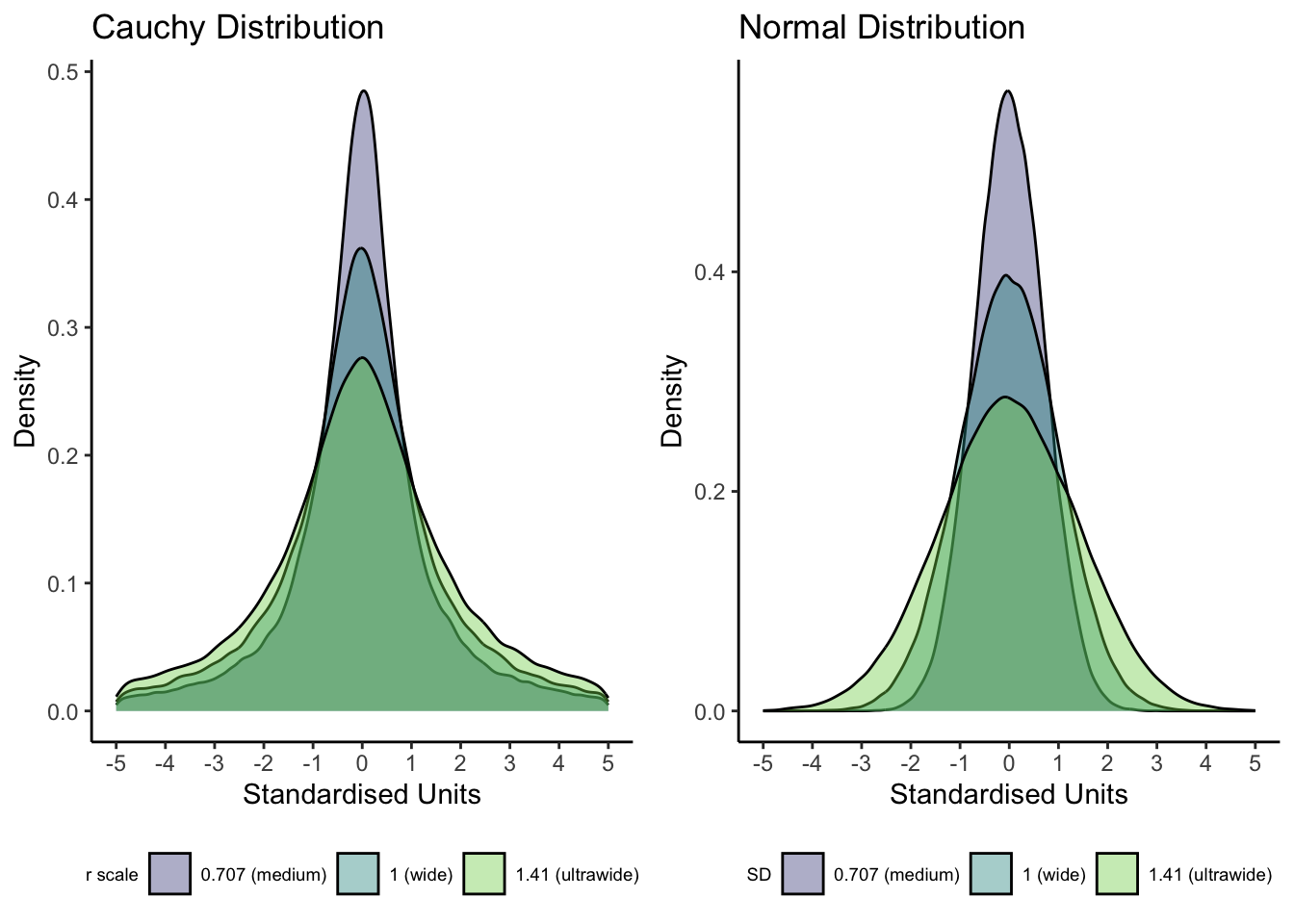
The default prior is set to "medium", but you could change this depending on your understanding of the area of research. See the function help page for different options here, but medium is equivalent to a value of 0.707 for scaling the Cauchy prior which is the default setting for most statistics software. You can interpret the r scale as 50% of the distribution covers values ± your chosen value. An effect of zero is the most likely, but the larger the r scale value, the more plausible you consider large effects. If you use a value of 0.707 ("medium") on a two-tailed test, this means 50% of the prior distribution covers values between ± 0.707. You can enter a numeric value for the precise scaling or there are a few word presets like "medium", "wide", and "ultrawide" depending on how strong or weak you want the prior to be.
Bastian_ttest <- ttestBF(formula = mean_bonding ~ CONDITION,
                        data = Bastian_data,
                        rscale = "medium",
                        paired = FALSE)
## Warning: data coerced from tibble to data frame
Bastian_ttest## Bayes factor analysis
## --------------
## [1] Alt., r=0.707 : 1.445956 ±0.01%
##
## Against denominator:
## Null, mu1-mu2 = 0
## ---
## Bayes factor type: BFindepSample, JZSDon't worry about the warning, there were just previous issues with using tibbles in the BayesFactor package. Now the package converts tibbles to normal R data frames before doing its thing.
With the medium prior, we have a Bayes factor of 1.45 (\(BF\)\(_1\)\(_0\) = 1.45), suggesting the experimental hypothesis is 1.45 times more likely than the point null hypothesis. By the guidelines from Wagenmakers et al. (2011), this is quite weak anecdotal evidence.
There is also a percentage next to the Bayes factor. This is the proportional error estimate and tells you the error in estimating the Bayes factor value. Less error is better and a rough rule of thumb is less than 20% is acceptable (Doorn et al., 2021). In this example, the error estimate is 0.01%, so very small. This means we could expect the Bayes factor to range between 1.44 and 1.45 which makes little impact on the conclusion.
4.4.1.1 Robustness check
This will be more important for modelling in the next chapter, but it is good practice to check the sensitivity of your results to your choice of prior. You would exercise caution if your choice of prior affects the conclusions you are making, such as weak evidence turning into strong evidence. If the qualitative conclusions do not change across plausible priors, then your findings are robust. For example, the Bayes factor for the Bastian et al. example decreases as the prior r scale increases.
| Prior | BayesFactor |
|---|---|
| Medium | 1.45 |
| Wide | 1.22 |
| Ultrawide | 0.97 |
A wider prior expresses less certainty about the size of the effect; larger effects become more plausible. Remember Bayes factors quantify the degree of belief in one hypothesis compared to another. As the evidence is quite weak, the Bayes factor decreases in favour of the null under weaker priors as you are expressing less certainty about the size of the effect.
4.4.1.2 One- vs two-tailed tests
The authors were pretty convinced that the pain group would score higher on the bonding rating than the control group, so lets see what happens with a one-tailed test to see how its done. We need to define the nullInterval argument to state we only consider negative effects.
Make sure you check the order of your groups to check which direction you expect the results to go in. If you expect group A to be smaller than group B, you would code for negative effects. If you expect group A to be bigger than group B, you would code for positive effects. A common mistake is defining the wrong direction if you do not know which order the groups are coded.
Bastian_onetail <- ttestBF(formula = mean_bonding ~ CONDITION,
                        data = Bastian_data,
                        rscale = "medium",
                        paired = FALSE,
                        nullInterval = c(-Inf, 0)) # negative only as we expect control < pain
## Warning: data coerced from tibble to data frame
Bastian_onetail## Bayes factor analysis
## --------------
## [1] Alt., r=0.707 -Inf<d<0 : 2.790031 ±0%
## [2] Alt., r=0.707 !(-Inf<d<0) : 0.1018811 ±0.02%
##
## Against denominator:
## Null, mu1-mu2 = 0
## ---
## Bayes factor type: BFindepSample, JZSIn a one-tailed test, we now have two tests. In row one, we have the test we want where we compare our experimental hypothesis (negative effects) against the point null. In row two, we have the opposite which is the complement of our experimental hypothesis, which would be that the effect is not negative. Even with a one-tailed test, the evidence in favour of our experimental hypothesis compared to the null is anecdotal at best (\(BF\)\(_1\)\(_0\) = 2.79).
If we wanted to test the null compared to the experimental hypothesis, we can simply take the reciprocal of the object, here demonstrated on the two-tailed object.
1 / Bastian_ttest## Bayes factor analysis
## --------------
## [1] Null, mu1-mu2=0 : 0.6915839 ±0.01%
##
## Against denominator:
## Alternative, r = 0.707106781186548, mu =/= 0
## ---
## Bayes factor type: BFindepSample, JZSFor this object, we already know there is anecdotal evidence in favour of the experimental hypothesis, so this is just telling us the null is less likely than the experimental hypothesis (\(BF\)\(_0\)\(_1\) = 0.69). This will come in handy when you specifically want to test the null though.
For the purposes of the rest of the demonstration, we will stick with our original object with a two-tailed test to see how we can interpret inconclusive results. In the original study, the pain group scored significantly higher than the control group, but the p-value was .048, so hardly convincing evidence. With Bayes factors, at least we can see we ideally need more data to make a decision.
4.4.1.3 Parameter estimation
We will spend more time on this process in week/chapter 10, but a Bayes factor on its own is normally not enough. We also want an estimate of the effect size and the precision around it. Within the BayesFactor package, there is a function to sample from the posterior distribution using MCMC sampling. We need to pass the t-test object into the posterior function, and include the number of iterations we want. We will use 10,000 here. Depending on your computer, this may take a few seconds.
If you use a one-tailed test, you must index the first object (e.g., Bastian_ttest[1]) as a one-tailed test includes two lines: 1) the directional alternative we state against the null and 2) the complement of the alternative against the null.
Bastian_samples <- posterior(Bastian_ttest,
                            iterations = 1e5) # 10,000 in math notation
Once we have the samples, we can use the base plot function to see trace plots (more on those in chapter 10) and a density plot of the posterior distributions for several parameters.
plot(Bastian_samples)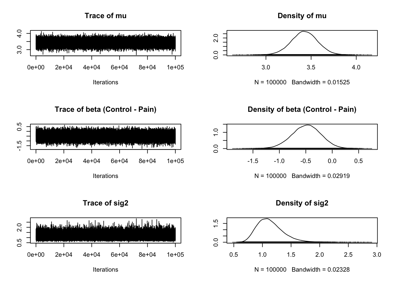
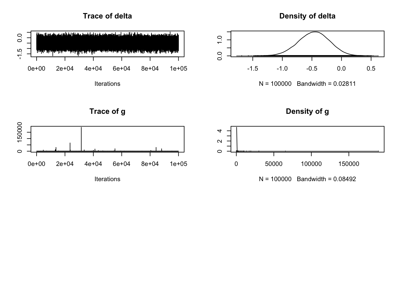
The second and fourth plots are what we are mainly interested in for a t-test. Once we know what kind of evidence we have for different hypotheses, typically we want to know what the effect size is. In the BayesFactor package, we get the mean difference between groups (unhelpfully named beta) and the effect size Delta, which is kind of like Cohen's d. It is calculated by dividing the t statistic by the square root of the sample size, so a type of standardised mean difference. One of my main complaints with the BayesFactor package is not explaining what the outputs mean as the only explanation I could find is old blog post with no clear overview in the documentation.
The plot provides the posterior distribution of different statistics based on sampling 10,000 times. For beta, we can see the peak of the distribution is around -0.5, spanning from above 0 to -1. For delta, we can see the peak of the distribution is around -0.5, and spans from above 0 to -1 again.
For a more fine-tuned description of the posterior distribution, we can use handy functions from the bayestestR package (Makowski et al., 2019). We will use this much more in chapter 10 as there are some great plotting functions, but these functions work for BayesFactor objects. To get the point estimates of each parameter, we can use the point_estimate function:
point_estimate(Bastian_samples)| Parameter | Median | Mean | MAP |
|---|---|---|---|
| mu | 3.4261304 | 3.4262019 | 3.4131426 |
| beta (Control - Pain) | -0.4848002 | -0.4892667 | -0.4665795 |
| sig2 | 1.1061817 | 1.1348647 | 1.0803148 |
| delta | -0.4619808 | -0.4664735 | -0.4443186 |
| g | 0.5448393 | 7.6797358 | 0.0236393 |
Our best guess (median of the posterior) for the mean difference between groups is -0.49 and a delta of -0.47 in favour of the pain group.
We do not just want a point estimate though, we also want the credible interval around it. For this, we have the hdi function.
hdi(Bastian_samples)| Parameter | CI | CI_low | CI_high |
|---|---|---|---|
| mu | 0.95 | 3.1355925 | 3.7088678 |
| beta (Control - Pain) | 0.95 | -1.0362104 | 0.0505082 |
| sig2 | 0.95 | 0.7316134 | 1.5957396 |
| delta | 0.95 | -0.9816252 | 0.0549678 |
| g | 0.95 | 0.0321040 | 7.7710573 |
So, 95% of the posterior distribution for the mean difference is between -1.04 and 0.04, and that delta is between -0.99 and 0.04. As both values cross 0, we would not be confident in these findings and ideally we would need to collect more data, which is consistent with the Bayes Factor results.
Finally, instead of separate functions, there is a handy wrapper for the median, 95% credible interval, and ROPE (more on that later).
describe_posterior(Bastian_samples)| Parameter | Median | CI | CI_low | CI_high | pd | ROPE_CI | ROPE_low | ROPE_high | ROPE_Percentage | |
|---|---|---|---|---|---|---|---|---|---|---|
| 4 | mu | 3.4261304 | 0.95 | 3.1373459 | 3.7109673 | 1.00000 | 0.95 | -0.1 | 0.1 | 0.0000000 |
| 1 | beta (Control - Pain) | -0.4848002 | 0.95 | -1.0426880 | 0.0452834 | 0.96438 | 0.95 | -0.1 | 0.1 | 0.0540526 |
| 5 | sig2 | 1.1061817 | 0.95 | 0.7707757 | 1.6676312 | 1.00000 | 0.95 | -0.1 | 0.1 | 0.0000000 |
| 2 | delta | -0.4619808 | 0.95 | -0.9985058 | 0.0413485 | 0.96438 | 0.95 | -0.1 | 0.1 | 0.0585263 |
| 3 | g | 0.5448393 | 0.95 | 0.0928315 | 15.8435212 | 1.00000 | 0.95 | -0.1 | 0.1 | 0.0076000 |
There are a bunch of tests and tricks we have not covered here, so check out the Bayesfactor package page online for a series of vignettes.
4.4.1.4 Reporting your findings
When reporting your findings, Doorn et al. (2021) suggest several key pieces of information to provide your reader:
A complete description and justification of your prior;
Clearly state each hypothesis you are comparing and specify using the Bayes factor notation (\(BF\)\(_0\)\(_1\) or \(BF\)\(_1\)\(_0\));
The Bayes factor value and error percentage;
A robustness check of your findings under different plausible priors;
Your parameter estimate (effect size) including the posterior mean or median and its 95% credible / highest density interval (HDI).
Where possible, try and provide the reader with the results in graphical and numerical form, such as including a plot of the posterior distribution. This will be easier in the next chapter as some of the plotting helper functions do not work nicely with the BayesFactor package.
4.4.2 Independent activity (Schroeder & Epley, 2015)
For an independent activity, we will use data from Schroeder & Epley (2015). The aim of the study was to investigate whether delivering a short speech to a potential employer would be more effective at landing you a job than writing the speech down and the employer reading it themselves. Thirty-nine professional recruiters were randomly assigned to receive a job application speech as either a transcript for them to read, or an audio recording of the applicant reading the speech.
The recruiters then rated the applicants on perceived intellect, their impression of the applicant, and whether they would recommend hiring the candidate. All ratings were originally on a Likert scale ranging from 0 (low intellect, impression etc.) to 10 (high impression, recommendation etc.), with the final value representing the mean across several items.
For this example, we will focus on the hire rating (variable "Hire_Rating" to see whether the audio condition would lead to higher ratings than the transcript condition (variable "CONDITION").
Schroeder_data <- read_csv("data/Schroeder_hiring.csv")

# Relabel condition to be more intuitive which group is which
Schroeder_data$CONDITION <- factor(Schroeder_data$CONDITION,
                                   levels = c(0, 1),
                                   labels = c("Transcript", "Audio"))
From here, apply what you learnt in the first guided example to this new independent task and complete the questions below to check your understanding. Since we expect higher ratings for audio than transcript, use a one-tailed test. Remember to sample from the posterior, so we can also get estimates of the effect sizes.
You can check your attempt to the solutions at the bottom of the page.
Schroeder_ttest <- NULLRounding to two decimals, what is the Bayes Factor in favour of the alternative hypothesis?
Looking at the guidelines from Wagenmakers et al. (2015), how could you describe the evidence in favour of the alternative hypothesis?
Rounding to two decimals, what is the absolute (ignoring the sign) mean difference (beta) in favour of the audio condition?
Looking at the 95% credible interval, can we rule out an effect of 0 given these data and model?
4.5 Bayes factors for two dependent samples
4.5.1 Guided example (Mehr et al., 2016)
For a paired samples t-test, the process is identical to the independent samples t-test apart from defining the variables. So, we will demonstrate a full example like before with less commentary, then you have an independent data frame to test your understanding.
The next study we are going to look at is by Mehr et al. (2016). They were interested in whether singing to infants conveyed important information about social affiliation. Infants become familiar with melodies that are repeated in their specific culture. The authors were interested in whether a novel person (someone they had never seen before) could signal to the child that they are a member of the same social group and attract their attention by singing a familiar song to them.
Mehr et al. (2016) invited 32 infants and their parents to participate in a repeated measures experiment. First, the parents were asked to repeatedly sing a previously unfamiliar song to the infants for two weeks. When they returned to the lab, they measured the baseline gaze (where they were looking) of the infants towards two unfamiliar people on a screen who were just silently smiling at them. This was measured as the proportion of time looking at the individual who would later sing the familiar song (0.5 would indicate half the time was spent looking at the familiar singer. Values closer to one indicate looking at them for longer). The two silent people on the screen then took it in turns to sing a lullaby. One of the people sung the song that the infant’s parents had been told to sing for the previous two weeks, and the other one sang a song with the same lyrics and rhythm, but with a different melody. Mehr et al. (2016) then repeated the gaze procedure to the two people at the start of the experiment to provide a second measure of gaze as a proportion of looking at the familiar singer.
We are interested in whether the infants increased the proportion of time spent looking at the singer who sang the familiar song after they sang, in comparison to before they sang to the infants. We have one dependent variable (gaze proportion) and one within-subjects independent variable (baseline vs test). We want to know whether gaze proportion was higher at test ("Test_Proportion_Gaze_to_Singer") than it was at baseline ("Baseline_Proportion_Gaze_to_Singer").
Mehr_data <- read_csv("data/Mehr_voice.csv") %>%
  select(Baseline = Baseline_Proportion_Gaze_to_Singer, # Shorten super long names
         Test = Test_Proportion_Gaze_to_Singer)

Mehr_ttest <- ttestBF(x = Mehr_data$Baseline,
                      y = Mehr_data$Test,
                      paired = TRUE,
                      rscale = "medium")

Mehr_ttest
## Bayes factor analysis
## --------------
## [1] Alt., r=0.707 : 2.296479 ±0%
##
## Against denominator:
## Null, mu = 0
## ---
## Bayes factor type: BFoneSample, JZSLike Bastian et al. (2014), we have just anecdotal evidence in favour of the experimental hypothesis over the null (\(BF\)\(_1\)\(0\) = 2.30).
Mehr et al. (2016) expected gaze proportion to be higher at test, so try defining a one-tailed test and see what kind of evidence we have in favour of the alternative hypothesis.
As before, we know there is only anecdotal evidence in favour of the experimental hypothesis, but we also want the effect size and its 95% credible interval. So, we can sample from the posterior, plot it, and get some estimates.
Mehr_samples <- posterior(Mehr_ttest,
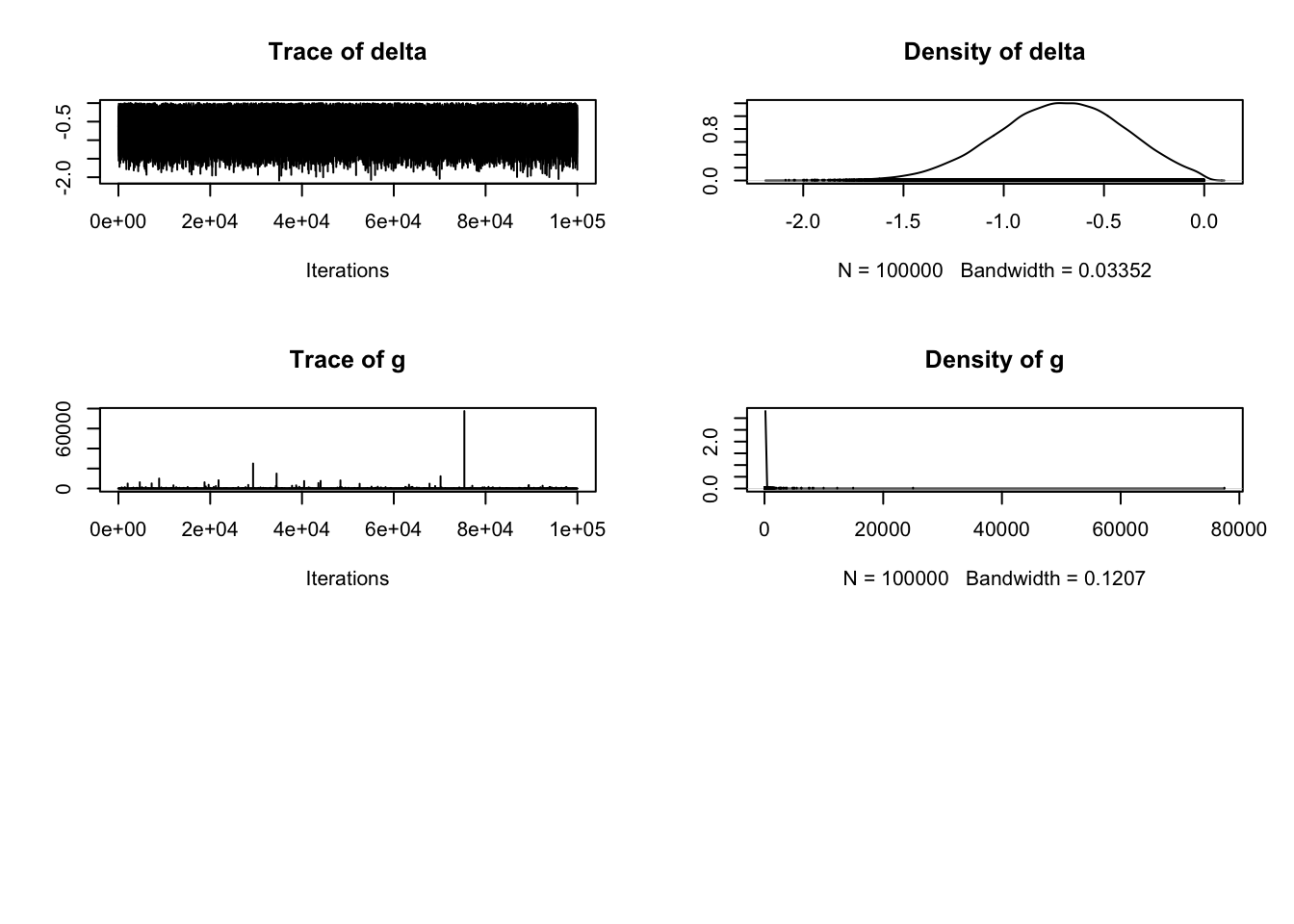
iterations = 1e5)Just note in the plot we have fewer panels as the paired samples approach simplifies things. Mu is our mean difference in the first panel and delta is our standardised effect in the third panel. For a dependent variable like gaze proportion, an unstandardised effect size is informative and comparable across studies, but its also useful to report standardised effect sizes for future power analyses etc.
# Subset first plot for mean to display correctly
plot(Mehr_samples[, 1],
     main = "Posterior for mu")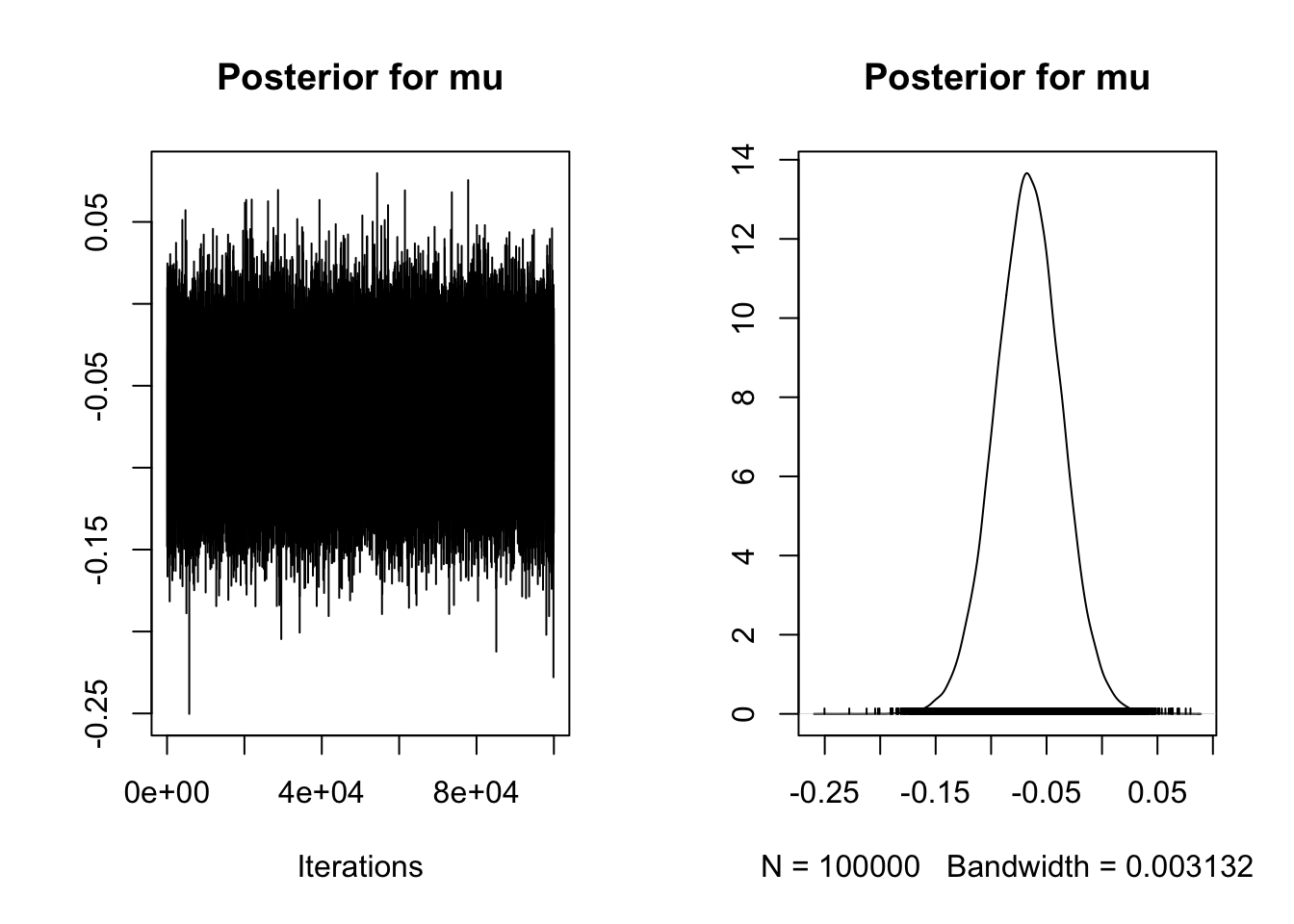
# Subset third plot for delta to display correctly
plot(Mehr_samples[, 3],
     main = "Posterior for delta")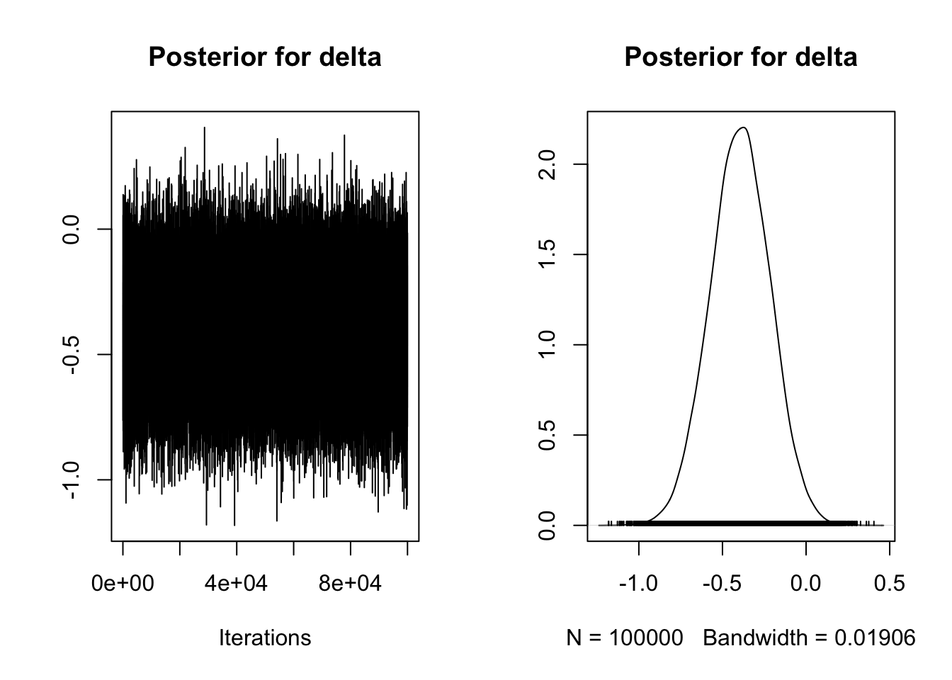
We finally have our wrapper function for the median posterior distribution and its 95% credible interval.
describe_posterior(Mehr_samples)| Parameter | Median | CI | CI_low | CI_high | pd | ROPE_CI | ROPE_low | ROPE_high | ROPE_Percentage | |
|---|---|---|---|---|---|---|---|---|---|---|
| 3 | mu | -0.0665270 | 0.95 | -0.1260660 | -0.0079075 | 0.9866 | 0.95 | -0.1 | 0.1 | 0.8898737 |
| 4 | sig2 | 0.0288372 | 0.95 | 0.0182590 | 0.0492998 | 1.0000 | 0.95 | -0.1 | 0.1 | 1.0000000 |
| 1 | delta | -0.3926439 | 0.95 | -0.7480745 | -0.0438846 | 0.9866 | 0.95 | -0.1 | 0.1 | 0.0260000 |
| 2 | g | 0.4905500 | 0.95 | 0.0877182 | 13.6082978 | 1.0000 | 0.95 | -0.1 | 0.1 | 0.0140421 |
We can see here the median posterior estimate of the mean difference is -.07 with a 95% credible interval ranging from -.13 to -.01. As the dependent variable is measured as a proportion of gaze time, infants looked at the familiar singer for 7% (1-13% for the 95% credible interval) longer at test than at baseline. This means we can exclude 0 from the likely effects, but we still only have anecdotal evidence in favour of the experimental hypothesis compared to the null.
4.5.2 Independent activity (Zwaan et al., 2020)
For your final independent activity, we have data from Zwaan et al. (2018) who wanted to see how replicable experiments from cognitive psychology are. For this exercise, we will explore the flanker task.
In short, we have two conditions: congruent and incongruent. In congruent trials, five symbols like arrows are the same and participants must identify the central symbol with a keyboard response. In incongruent trials, the four outer symbols are different to the central symbol. Typically, we find participants respond faster to congruent trials than incongruent trials. The dependent variable here is the mean response time in milliseconds (ms).
We want to know whether response times are faster to congruent trials ("session1_responsecongruent") than incongruent trials ("session1_incongruent"). Zwaan et al. measured a few things like changing the stimuli and repeating the task in two sessions, so we will just focus on the first session for this example.
Perform a paired samples t-test comparing the response times to congruent and incongruent trials. The questions below relate to a one-tailed test since there is a strong prediction to expect faster responses in the congruent condition compared to the incongruent condition. Think carefully about whether you expect positive or negative effects depending on the order you enter the variables.
You can check your attempt to the solutions at the bottom of the page.
Zwaan_data <- read_csv("data/Zwaan_flanker.csv")

Zwaan_ttest <- NULL- Looking at the guidelines from Wagenmakers et al. (2011), how could you describe the evidence in favour of the alternative hypothesis?
The Bayes Factor for this analysis is huge. Unless you edit the settings, R reports large numbers in scientific notation. The Bayes Factor in favour of the alternative hypothesis here is 8.7861e+12 or as a real number 8786100000000. For a finding as established as the flanker task, testing against a point null is not too informative, but this shows what extreme evidence looks like. We will come back to this in the ROPE demonstration later.
Rounding to two decimals, what is the absolute (ignoring the sign) mean difference (beta) in response time between congruent and incongruent trials?
Looking at the 95% credible interval for mu, we would expect the absolute mean difference to range between ms and ms.
Rounding to two decimals, what is the absolute standardised mean difference (delta) in response time between congruent and incongruent trials?
4.6 Equivalence Testing vs ROPE
4.6.1 Guided example for two independent samples (Bastian et al., 2014)
In sections 9.4 and 9.5, we focused on the Bayesian approach to null hypothesis testing. We compared the alternative hypothesis to the null hypothesis and wanted to know how much we should shift our beliefs. However, there are times when comparing against a point null is uninformative. The same advice applies to frequentist statistics where you can use equivalence testing (see the bonus section in the appendix if you are interested in this). In this setup, you set two boundaries representing your smallest effect size of interest (SESOI) and conduct a two one-sided test: one comparing your sample mean (difference) to the upper bound and one comparing your sample mean (difference) to the lower bound. If both tests are significant, you can conclude the mean was within your bounds and it is practically equivalent to zero.
In a Bayesian framework, we follow a similar approach by setting an upper and lower bound for the interval we consider practically or theoretically meaningful. This is known as the Region of Practical Equivalence (ROPE). However, we do not perform a two one-sided test, we directly compare the posterior distribution to the ROPE and interpret how much of the ROPE captures our 95% credible interval. This creates three decisions (Kruschke & Liddell, 2018a) instead of comparing the experimental hypothesis to the point null:
HDI completely outside the ROPE: We reject the ROPE as the parameter is larger than the effects we consider too small to be practically/theoretically meaningful.
HDI completely within the ROPE: We accept the ROPE as the parameter is smaller than the effects we consider practically/theoretically meaningful.
HDI and the ROPE partially overlap: We are undecided as we need more data and greater precision in the posterior to make a decision about whether we can reject the ROPE.
This will be more meaningful in chapter 10 when we turn to Bayesian modelling as the bayestestR package has great functions for visualising the ROPE, but they unfortunately do not work with BayesFactor objects. We will return to the Bastian et al. (2014) data and the describe_posterior() function. If you explored the complete output earlier, you might have noticed the values relating to ROPE, but we ignored it at the time. As a reminder, lets see the output:
# rerun the code from section 9.4.1 if you do not have this object saved
describe_posterior(Bastian_samples)| Parameter | Median | CI | CI_low | CI_high | pd | ROPE_CI | ROPE_low | ROPE_high | ROPE_Percentage | |
|---|---|---|---|---|---|---|---|---|---|---|
| 4 | mu | 3.4261304 | 0.95 | 3.1373459 | 3.7109673 | 1.00000 | 0.95 | -0.1 | 0.1 | 0.0000000 |
| 1 | beta (Control - Pain) | -0.4848002 | 0.95 | -1.0426880 | 0.0452834 | 0.96438 | 0.95 | -0.1 | 0.1 | 0.0540526 |
| 5 | sig2 | 1.1061817 | 0.95 | 0.7707757 | 1.6676312 | 1.00000 | 0.95 | -0.1 | 0.1 | 0.0000000 |
| 2 | delta | -0.4619808 | 0.95 | -0.9985058 | 0.0413485 | 0.96438 | 0.95 | -0.1 | 0.1 | 0.0585263 |
| 3 | g | 0.5448393 | 0.95 | 0.0928315 | 15.8435212 | 1.00000 | 0.95 | -0.1 | 0.1 | 0.0076000 |
For more information on ROPE within the bayestestR package, see the online vignettes. In the output, we have:
The 95% credible interval - we will need this to compare to the ROPE.
The probability of direction (pd) - how much of the posterior distribution is in a positive or negative direction?
Region of practical equivalence (ROPE) - the interval we would consider for our SESOI.
% in ROPE - how much of the posterior is within the ROPE?
By default, the describe_posterior() function sets the ROPE region to the mean plus or minus 0.1 * SD of your response. We can set our own ROPE using the rope_range argument. Justifying your ROPE is probably the most difficult decision you will make as it requires subject knowledge for what you would consider the smallest effect size of interest. From the lecture, there are different strategies:
Your understanding of the applications / mechanisms (e.g., a clinically meaningful decrease in pain).
Smallest effects from previous research (e.g., lower bound of individual study effect sizes or lower bound of a meta-analysis).
Small telescopes (the effect size the original study had 33% power to detect).
For Bastian et al. (2014), they measured bonding on a 5-point Likert scale, so we might consider anything less than a one-point difference as too small to be practically meaningful.
describe_posterior(Bastian_samples,
rope_range = c(-1, 1)) # plus or minus one point difference| Parameter | Median | CI | CI_low | CI_high | pd | ROPE_CI | ROPE_low | ROPE_high | ROPE_Percentage | |
|---|---|---|---|---|---|---|---|---|---|---|
| 4 | mu | 3.4261304 | 0.95 | 3.1373459 | 3.7109673 | 1.00000 | 0.95 | -1 | 1 | 0.0000000 |
| 1 | beta (Control - Pain) | -0.4848002 | 0.95 | -1.0426880 | 0.0452834 | 0.96438 | 0.95 | -1 | 1 | 0.9898737 |
| 5 | sig2 | 1.1061817 | 0.95 | 0.7707757 | 1.6676312 | 1.00000 | 0.95 | -1 | 1 | 0.2915789 |
| 2 | delta | -0.4619808 | 0.95 | -0.9985058 | 0.0413485 | 0.96438 | 0.95 | -1 | 1 | 1.0000000 |
| 3 | g | 0.5448393 | 0.95 | 0.0928315 | 15.8435212 | 1.00000 | 0.95 | -1 | 1 | 0.6907789 |
Note how changing the ROPE range changes the values for every parameter, so you will need to think which parameter you are interested in and what would be a justifiable ROPE for it. For this example, we will focus on the mean difference between groups (beta). Using a ROPE of plus or minus 1, 99.26% of the 95% HDI is within the ROPE. Its so close, but it falls in the third decision from above where we need more data to make a decision. The lower bound of the HDI is -1.03, so it extends just outside our ROPE region.
Compared to the standard Bayes factor where we had weak evidence in favour of the alternative hypothesis compared to the point null, using the ROPE approach means we also have an inconclusive decision, but our effect size is almost too small to be practically meaningful.
4.6.2 Independent activity for two independent samples (Schroeder & Epley, 2014)
For this activity, you will need the objects you created in section 9.4.2 for the independent activity. Remember it is based on a one-tailed t-test as we expected higher ratings for the audio group compared to the transcript group. You will need the samples from the posterior as the only thing you will need to change is the arguments you use in the describe_posterior() function.
Use the describe_posterior() from section 9.4.2, but this time enter values for the ROPE arguments. The original study was on a 10-point scale. Your choice of ROPE will depend on your understanding of the subject area, but they measured their outcomes on a 0-10 scale. We might have a higher bar for concluding a meaningful effect of medium on people's hire ratings, so use a ROPE region of 2 points. Since we used a one-tailed test focusing on negative effects (transcript < audio), we can just focus on the region between -2 and 0.
You can check your attempt to the solutions at the bottom of the page.
Looking at the 95% credible interval for beta, we would expect the absolute mean difference to range between and .
Rounding to two decimals, what percentage of the 95% credible interval is within the ROPE?
-
What is the most appropriate conclusion based on this ROPE?:
4.6.3 Guided example for two dependent samples (Mehr et al., 2014)
For the Mehr et al. (2014) data, the outcome is a little easier to interpret for an unstandardised effect than the two between-subjects examples. They compared infants' proportion of gaze duration spent on the model that sang the familiar song and wanted to know whether this would increase at test compared to baseline. As the proportion of gaze is bound between 0 (none of the time) to 1 (all of the time), we might consider a 5% (0.05) increase or decrease as theoretically meaningful if we are not very certain the test will be higher than baseline.
describe_posterior(Mehr_samples,
rope_range = c(-0.05, 0.05))| Parameter | Median | CI | CI_low | CI_high | pd | ROPE_CI | ROPE_low | ROPE_high | ROPE_Percentage | |
|---|---|---|---|---|---|---|---|---|---|---|
| 3 | mu | -0.0665270 | 0.95 | -0.1260660 | -0.0079075 | 0.9866 | 0.95 | -0.05 | 0.05 | 0.2747263 |
| 4 | sig2 | 0.0288372 | 0.95 | 0.0182590 | 0.0492998 | 1.0000 | 0.95 | -0.05 | 0.05 | 1.0000000 |
| 1 | delta | -0.3926439 | 0.95 | -0.7480745 | -0.0438846 | 0.9866 | 0.95 | -0.05 | 0.05 | 0.0022842 |
| 2 | g | 0.4905500 | 0.95 | 0.0877182 | 13.6082978 | 1.0000 | 0.95 | -0.05 | 0.05 | 0.0000000 |
Our observed mean difference was a posterior median of -0.07, 95% CI = [-.13, -0.01], which is 27.50% within the ROPE region of plus or minus 0.05 points. We are not far off ruling out our ROPE, but we still need more data to make a decision. Hopefully, you can see by this point, many of these studies have more inconclusive conclusions when analysed through a Bayesian framework than the original frequentist statistics.
4.6.4 Independent activity for two dependent samples (Zwaan et al., 2018)
For this activity, you will need the objects you created in section 9.5.2 for the independent activity. Remember it is based on a one-tailed t-test as we expected faster response times to congruent trials than incongruent trials. You will need the samples from the posterior as the only thing you will need to change is the arguments you use in the describe_posterior() function.
Use the describe_posterior() from section 9.5.2, but this time enter values for the ROPE arguments. Set your ROPE to -10-0ms (or 0-10 depending on the order you entered the variables) as these are smaller effects closer to the sampling error we can expect with response time experiments held online (Reimers & Stewart, 2015).
You can check your attempt to the solutions at the bottom of the page.
Looking at the 95% credible interval for mu, we would expect the absolute mean difference to range between and .
What percentage of the 95% credible interval is within the ROPE?
-
What is the most appropriate conclusion based on this ROPE?:
4.7 Summary
In this chapter, you learnt about hypothesis testing using a Bayesian framework. The first two activities explored the logic of Bayesian statistics to make inferences and how it can be used to test hypotheses when expressed as the Bayes factor. You then learnt how to perform Bayes factors applied to the simplest cases of two independent samples and two dependent samples. Bayes factors are a useful way of quantifying the evidence in favour of a hypotheses compared to a competing hypothesis. Bayesian statistics can still be used mindlessly, but hopefully you can see they provide the opportunity to move away from purely dichotomous thinking. Evidence that would be statistically significant (p < .05) but close to alpha only represents anecdotal evidence.
As with any new skill, practice is the best approach to becoming comfortable in applying your knowledge to novel scenario. Hopefully, you worked through the guided examples and tested your understanding on the independent activities.
For further learning, we recommend the following resources relevant to this chapter:
Doorn et al. (2021) - Although it focuses on the JASP software, this article provides an accessible introduction to Bayes factors and how you can report your findings.
Kruschke & Liddell (2018b) - This article discusses the proposed shift away from dichotomous hypothesis testing towards estimation and how it relates to Bayesian statistics through summarising the posterior and the ROPE procedure.
Wong et al. (2021) - Although Bayes factors have the potential to help you make more nuanced inferences, they are still prone to misinterpretations. This preprint outlines common errors and misconceptions when researcher report Bayes factors.
4.8 Independent activity solutions
4.8.1 Schroeder and Epley (2015) Bayes factor
Schroeder_ttest <- ttestBF(formula = Hire_Rating ~ CONDITION,
        data = Schroeder_data,
        rscale = "medium",
        nullInterval = c(-Inf, 0)) # Expect negative effects since Transcript < Audio
## Warning: data coerced from tibble to data frame
Schroeder_ttest## Bayes factor analysis
## --------------
## [1] Alt., r=0.707 -Inf<d<0 : 8.205739 ±0%
## [2] Alt., r=0.707 !(-Inf<d<0) : 0.1020371 ±0%
##
## Against denominator:
## Null, mu1-mu2 = 0
## ---
## Bayes factor type: BFindepSample, JZS
# We need to index the first object as a one-tailed test includes two lines:
# 1. Directional alternative we state against the null
# 2. Complement of the alternative against the null

Schroeder_samples <- posterior(Schroeder_ttest[1],
                               iterations = 1e5)
plot(Schroeder_samples)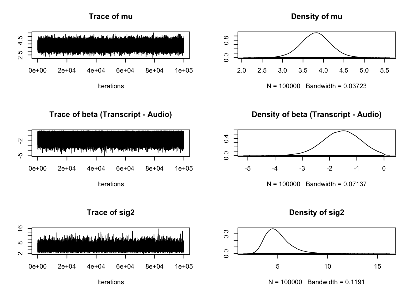
describe_posterior(Schroeder_samples)| Parameter | Median | CI | CI_low | CI_high | pd | ROPE_CI | ROPE_low | ROPE_high | ROPE_Percentage | |
|---|---|---|---|---|---|---|---|---|---|---|
| 4 | mu | 3.8130925 | 0.95 | 3.109169 | 4.5185592 | 1 | 0.95 | -0.1 | 0.1 | 0 |
| 1 | beta (Transcript - Audio) | -1.5465217 | 0.95 | -2.946880 | -0.3121002 | 1 | 0.95 | -0.1 | 0.1 | 0 |
| 5 | sig2 | 4.7849364 | 0.95 | 3.138439 | 7.8110282 | 1 | 0.95 | -0.1 | 0.1 | 0 |
| 2 | delta | -0.7084995 | 0.95 | -1.362898 | -0.1365876 | 1 | 0.95 | -0.1 | 0.1 | 0 |
| 3 | g | 0.7529274 | 0.95 | 0.113435 | 21.8814934 | 1 | 0.95 | -0.1 | 0.1 | 0 |
4.8.2 Zwaan et al. (2020) Bayes factor
Zwaan_ttest <- ttestBF(x = Zwaan_data$session1_responsecongruent,
                      y = Zwaan_data$session1_incongruent,
                      paired = TRUE,
                      rscale = "medium",
                      nullInterval = c(-Inf, 0)) # negative as we expect incongruent to be larger than congruent

Zwaan_ttest
## Bayes factor analysis
## --------------
## [1] Alt., r=0.707 -Inf<d<0 : 8.786135e+12 ±0%
## [2] Alt., r=0.707 !(-Inf<d<0) : 60.58291 ±0%
##
## Against denominator:
## Null, mu = 0
## ---
## Bayes factor type: BFoneSample, JZS
Zwaan_samples <- posterior(Zwaan_ttest[1], # index first item for a one-tailed test
                          iterations = 1e5)
plot(Zwaan_samples[, 1],
     main = "Posterior for mu")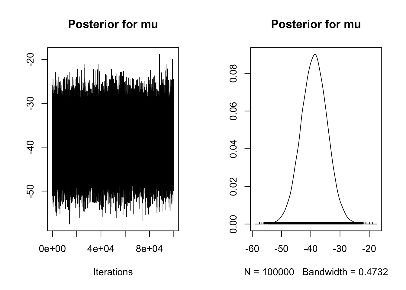
plot(Zwaan_samples[, 3],
     main = "Posterior for delta")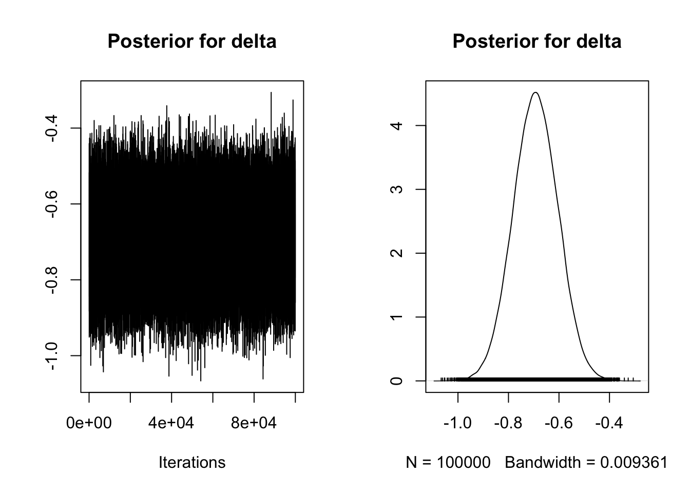
describe_posterior(Zwaan_samples)| Parameter | Median | CI | CI_low | CI_high | pd | ROPE_CI | ROPE_low | ROPE_high | ROPE_Percentage | |
|---|---|---|---|---|---|---|---|---|---|---|
| 3 | mu | -38.7918762 | 0.95 | -47.6011164 | -30.0234377 | 1 | 0.95 | -0.1 | 0.1 | 0 |
| 4 | sig2 | 3146.1775444 | 0.95 | 2548.8931250 | 3953.1759593 | 1 | 0.95 | -0.1 | 0.1 | 0 |
| 1 | delta | -0.6923077 | 0.95 | -0.8652760 | -0.5196815 | 1 | 0.95 | -0.1 | 0.1 | 0 |
| 2 | g | 0.7060218 | 0.95 | 0.1296344 | 19.6262419 | 1 | 0.95 | -0.1 | 0.1 | 0 |
4.8.3 Schroeder and Epley (2015) ROPE
describe_posterior(Schroeder_samples,
rope_range = c(-2, 0))| Parameter | Median | CI | CI_low | CI_high | pd | ROPE_CI | ROPE_low | ROPE_high | ROPE_Percentage | |
|---|---|---|---|---|---|---|---|---|---|---|
| 4 | mu | 3.8130925 | 0.95 | 3.109169 | 4.5185592 | 1 | 0.95 | -2 | 0 | 0.0000000 |
| 1 | beta (Transcript - Audio) | -1.5465217 | 0.95 | -2.946880 | -0.3121002 | 1 | 0.95 | -2 | 0 | 0.7561895 |
| 5 | sig2 | 4.7849364 | 0.95 | 3.138439 | 7.8110282 | 1 | 0.95 | -2 | 0 | 0.0000000 |
| 2 | delta | -0.7084995 | 0.95 | -1.362898 | -0.1365876 | 1 | 0.95 | -2 | 0 | 1.0000000 |
| 3 | g | 0.7529274 | 0.95 | 0.113435 | 21.8814934 | 1 | 0.95 | -2 | 0 | 0.0000000 |
4.8.4 Zwaan et al. (2020) ROPE
describe_posterior(Zwaan_samples,
rope_range = c(-10, 0))| Parameter | Median | CI | CI_low | CI_high | pd | ROPE_CI | ROPE_low | ROPE_high | ROPE_Percentage | |
|---|---|---|---|---|---|---|---|---|---|---|
| 3 | mu | -38.7918762 | 0.95 | -47.6011164 | -30.0234377 | 1 | 0.95 | -10 | 0 | 0 |
| 4 | sig2 | 3146.1775444 | 0.95 | 2548.8931250 | 3953.1759593 | 1 | 0.95 | -10 | 0 | 0 |
| 1 | delta | -0.6923077 | 0.95 | -0.8652760 | -0.5196815 | 1 | 0.95 | -10 | 0 | 1 |
| 2 | g | 0.7060218 | 0.95 | 0.1296344 | 19.6262419 | 1 | 0.95 | -10 | 0 | 0 |