22 Reporting Power Analyses and Reporting Correlation Results
In this research skills chapter, we will explore two topics. The first on reporting power analyses relates to the method section we covered prior to reading week. A power analysis to justify how many participants you require for your study is typically included in the participants or data analysis sub-section of the method. However, because of the schedule, there are topics we must cover before exploring power in greater detail. This means if you are reading this section in week 7, you have not had the lecture or data skills chapter on power yet. We wanted to make sure we cover reporting power though for anyone who wants to go above and beyond in the stage one group report.
If you have not explored power analysis in your independent reading yet, you can skip to the structure of the results section which is our second topic. We will cover key content to include and details on APA formatting for results. This week, we focus more reporting correlation results, then we will cover t-test results and data visualisation in week 8.
22.1 Reporting power analyses
In this section, we will recap the concept of statistical power, outline different options for choosing your smallest effect size of interest, reporting your power analysis, and finally preparing for a difference between your planned sample size and your final sample size.
22.1.1 Recommended resources to revise statistical power
-
In semester 1, the concept of statistical power and how it applies to specific statistical tests are spread across several weeks:
Week 4 - Hypothesis testing
Week 5 - Power applied to correlations
Week 7 - Power applied to t-tests
Chapter 11 of the PsyTeachR book Fundamentals of Quantitative Analysis outlines how to perform power analysis in R for different statistical tests.
Bartlett and Charles (2022) provide a beginner's tutorial to power analysis. Part 1 outlines the concept of statistical power and part 2 discusses justifying the inputs you use in power analysis. Ignore part 3 as you will be using R instead of jamovi.
22.1.2 Statistical power recap
In null hypothesis significance testing (NHST), we can put a limit on two types of error. Type I errors (false positives) are when we reject the null hypothesis and conclude a test was statistically significant, when really the null hypothesis is true. Type II errors (false negatives) are when we retain the null hypothesis and conclude a test was non-significant, when really the null hypothesis is false.
Statistical power is related to the second type of error (type II). The definition of power is the long run probability of your study design correctly rejecting the null hypothesis when there is a true effect to be found. In short, "if an effect exists, how likely am I to detect it"? If a study has high statistical power, you would reliably detect a given effect size. If a study has low statistical power, you would not reliably detect a given effect size.
In null hypothesis significance testing, there are four key concepts:
Alpha: The predetermined cut-off in your design at which you reject the null hypothesis (normally set at \(\alpha\) = .05). This is your false positive error rate to limit the number of type I errors you would be willing to make.
Power: The ability of a design to find an effect based on 1 - \(\beta\), where beta is normally set at .20 or .10, producing power = .80 or .90. Beta is the false negative error rate to limit the number of type II errors you would be willing to make.
Effect size: A number that expresses the magnitude of the phenomenon related to your research question. This will typically be Cohen's d for the standardised mean difference in t-tests or the correlation coefficient r.
Sample size: The number of participants or observations in your study.
Conveniently, there is an interaction between the four key concepts of Alpha, Power, Effect Size, and Sample Size (APES). If you state three, you can calculate the fourth. Assuming you use the field standards of \(\alpha\) = .05 and power = .80, choosing the final input of sample size or effect size produces one of two informative types of power analysis:
A priori power analysis: You solve power analysis for the number of participants you need for a given value of \(\alpha\), power, and effect size.
Sensitivity power analysis: You solve power analysis for the effect size you can detect for a given value of \(\alpha\), power, and sample size.
For an example, Mehr et al. (2016, pg. 487) report the following a priori power analysis in their study on the effect of melody on infants:
"Statistical power. The target sample size of 32 was determined before the experiment began, to ensure adequate power to detect a positive selective-attention effect. A similar experiment testing effects of language rather than music (Kinzler et al., 2007) obtained an effect size (d) of 0.54, and a sample of 32 had .84 power to detect an effect of this magnitude."
We can reproduce their power analysis using the pwr package for a paired samples t-test (if you have not got to week 8 in data skills yet, do not worry if this looks unfamiliar):
pwr.t.test(d = 0.54,
           sig.level = .05,
           power = .84,
           type = "paired",
           alternative = "two.sided")
##
## Paired t test power calculation
##
## n = 31.91057
## d = 0.54
## sig.level = 0.05
## power = 0.84
## alternative = two.sided
##
## NOTE: n is number of *pairs*Since we left the argument n blank, we receive that as the output of our a priori power analysis. We need 31.91 participants, but we always round up to a whole number of participants to avoid underestimating, so we would need 32 participants. The power analysis in Mehr et al. provides one example, but it is not perfect. There are some inputs they do not explicitly specify, so we will return to this example in reporting your power analysis below.
For your stage one report (and looking forward to your dissertation), you could report an a priori power analysis to inform how many participants you would need to detect your smallest effect size of interest. Power analysis and pre-registration is most informative in the design phase of research, so you would typically perform a power analysis to inform how many participants you try and recruit.
Just keep in mind: for the assignment in RM1 you have no control over the final sample size as we collected data for you. This means there might be a difference in your planned sample size from the a priori power analysis and the final sample size you work with. Therefore, we have a section on sensitivity power analysis to consider potential differences in your planned vs final sample size.
22.1.3 Choosing a smallest effect size of interest
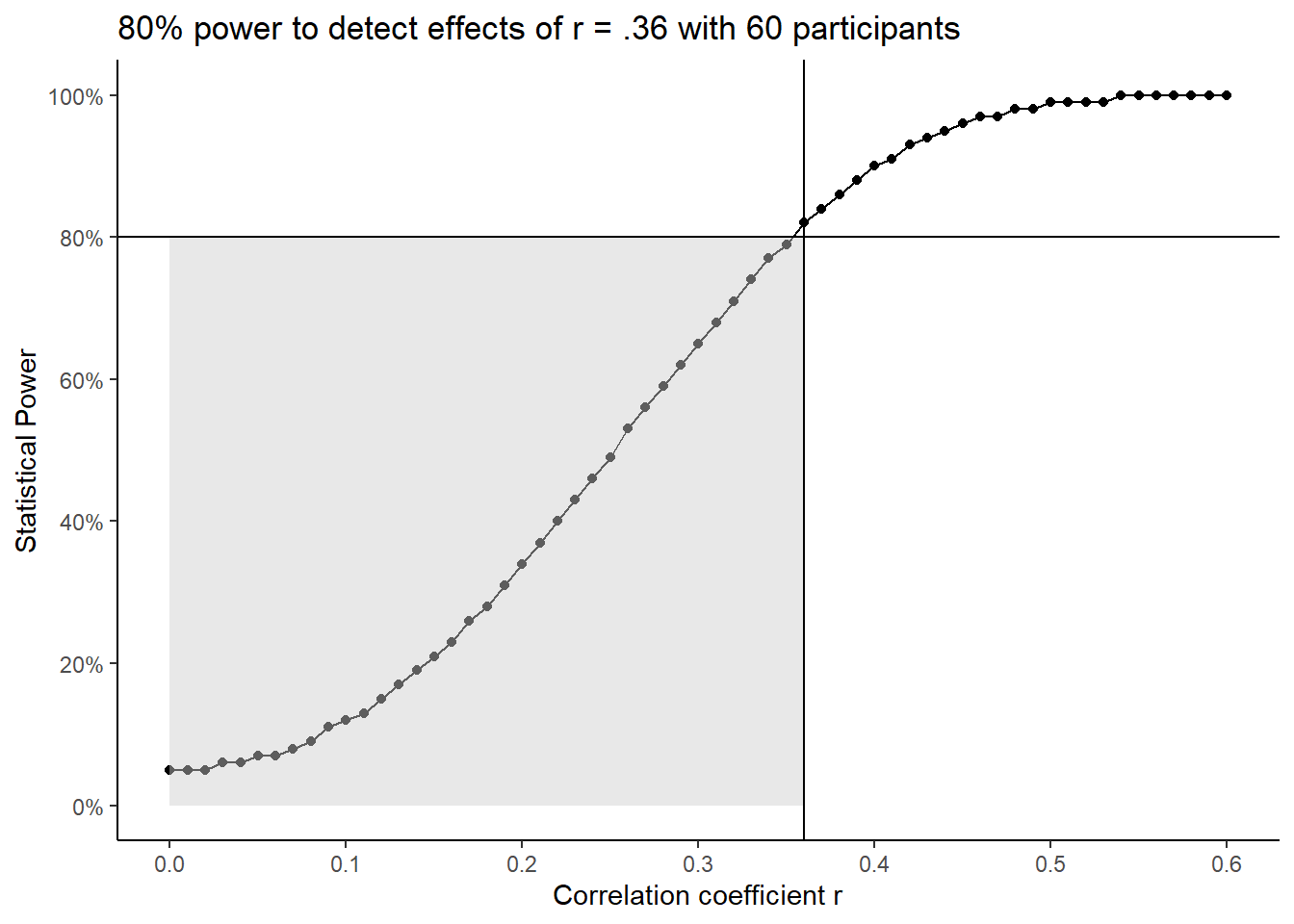
For an a priori power analysis, you need to enter an effect size. The term we use for this is the smallest effect size of interest. It is rare you would know precisely what effect size you were looking for - as you would not need the study if you understood the topic that well. This means your smallest effect size of interest represents the threshold for what effect sizes you want your study sensitive enough to detect. Power exists along a curve, so holding the sample size and all other inputs constant, you would be less likely to detect smaller effects, but more likely to detect effects larger than your smallest effect of interest.
The following plot is a power curve showing the relationship between the correlation coefficient r as the effect size and statistical power for a given sample size. Assuming our power analysis suggested we need to collect 60 participants, we would have 80% power to detect effects of r = .36. The smallest effect size of interest is where the two lines meet for your desired level of power (here 80%). As you move down the curve highlighted by the grey region, you would be less likely to detect effects smaller than your smallest effect size of interest. As you move up the curve, you would be more likely to detect effects larger than your smallest effect size of interest. In short, and assuming you want to keep power at 80% or higher, then you would be looking for effect sizes at, or greater than, your smallest effect size of interest.
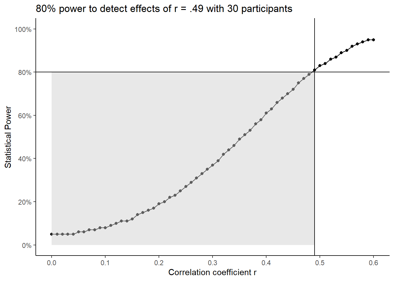
To demonstrate what this looks like for a larger smallest effect size of interest, if your power analysis suggested we need 30 participants, we would have 80% power to detect effects of r = .49. The smallest effect size of interest is again represented by where the two lines meet. Since we only wanted our design to be sensitive to larger effects, there is a larger grey region to highlight the effects we would be less likely to detect. As you move down the curve, you would be less likely to detect effects smaller than r = .49. As you move up the curve, you would be more likely to detect effects larger than r = .49. In short, you would be still be looking for effect sizes at, or greater than, your smallest effect size of interest, but that threshold shifts to exclude a larger region of smaller effects.
Assuming you use the field standards of \(\alpha\) = .05 and power = .80, this leaves the smallest effect size of interest as the main decision you must make. Choosing an effect size is the hardest part of power analysis, but there is no one correct answer, only a difference between justified and unjustified. In your power analysis, we care more about your justification for your choice of effect size rather than the value itself.
You could always aim for a tiny effect size but in a real study you are trying to compromise between an informative study and the resources (time / money) you have available. You could always aim for a large effect size, but you might miss potentially informative smaller effects. This means you must choose your smallest effect size of interest based on your understanding of the topic area and consider what effects you would not want to miss out on.
There are different strategies for choosing a smallest effect size of interest (see Lakens, 2022 for a full discussion):
Individual published studies: What effect sizes do similar studies to yours report?
Meta-analyses: What is the average effect size across several studies on a topic?
Effect size distributions: For a given topic, what is the distribution of effect sizes for what is considered small, medium, and large?
22.1.4 Reporting your power analysis
If you do report a power analysis, think about what information would allow the reader to reproduce your power analysis and understand your justification behind each input. Bakker et al. (2020) reviewed power analyses reported in pre-registrations and review boards and highlighted the most common omissions. From a sample of 210 studies, the most common omissions (% is the percentage of studies missing the information) in the features of a power analysis were:
Sidedness of the test (78%)
Justification for effect size (45%)
Type of effect size (30%)
Alpha value (29%)
Value of effect size (15%)
Power / beta value (15%)
Sample size (8%)
Bakker et al. observed that the most common omission was whether researchers assumed a one- or two-tailed test and the least common omission was the sample size the power analysis suggested.
Previously, we highlighted that Mehr et al. does not provide a complete example of reporting a power analysis. As an activity, we would like you to work through different adaptations we prepared and indicate what information you think is included and what you think is missing. Each adaptation is hidden behind a "show me" tab, so you can view each one in turn and focus on asking yourself what information is missing. We will compare each adaptation side by side afterwards.
22.1.4.1 Adaptation one
Using the field standards of power = .80 and alpha = .05, and an effect size from previous studies, we will require 29 infants in our study.
In adaptation one, what information do you think is missing?
Sidedness of the test?
Justification for effect size?
Type of effect size?
Alpha value?
Value of the effect size?
Power / beta value?
Sample size?
22.1.4.2 Adaptation two
Previous related research looking into how infants can develop and show selective-attention suggested a medium sized effect. As such, using the field standards of power = .80 and alpha = .05, and d = 0.54, we will require 29 infants in our study.
In adaptation two, what information do you think is missing?
Sidedness of the test?
Justification for effect size?
Type of effect size?
Alpha value?
Value of the effect size?
Power / beta value?
Sample size?
22.1.4.3 Adaptation three
Previous related research looking into how infants can develop and show selective-attention through music (Mehr et al., 2016) and language (Kinzler et al., 2007) suggested a medium sized effect around d = 0.54. As such, using the field standards of power = .80 and alpha = .05, and the suggested effect size from previous studies, we will require 29 infants in our study for a two-tailed test.
Sidedness of the test?
Justification for effect size?
Type of effect size?
Alpha value?
Value of the effect size?
Power / beta value?
Sample size?
22.1.4.4 Activity summary
Adaptation 3 is by no means a perfect example. The justification for the effect size could be more detailed and there are some subtle details Bakker et al. (2020) did not assess in their review. For example, you could mention the statistical test it is based on for absolutely clarity, and justify using the field standard values for alpha and power. To highlight how each adaptation changes, we will start with number one which included the fewest details and it would be difficult to reproduce the power analysis.
Using the field standards of power = .80 and alpha = .05, and an effect size from previous studies, we will require 29 infants in our study.
We only have the field standards of 80% power, 5% alpha, and we need 29 participants. There is no mention of the effect size, no justification, and no mention of the test it is based on.
Adding bold to adaptation two, we add more details.
Previous related research looking into how infants can develop and show selective-attention suggested a medium sized effect. As such, using the field standards of power = .80 and alpha = .05, and d = 0.54, we will require 29 infants in our study.
We mention studies on this topic report a medium sized effect, so that could be our smallest effect size of interest. We then specify an effect of d = 0.54 to add another input for our power analysis. However, we are vague about the studies that report the effect and there is no mention of the test or the number of tails it is based on.
Adding a final round of bold to adaptation three, we add a few more details.
Previous related research looking into how infants can develop and show selective-attention through music (Mehr et al., 2016) and language (Kinzler et al., 2007) suggested a medium sized effect around d = 0.54. As such, using the field standards of power = .80 and alpha = .05, and the suggested effect size from previous studies, we will require 29 infants in our study for a two-tailed test.
This time, the explanation could be more detailed for why this value represents the smallest effect size of interest, but we outlined studies to support this decision. We add the number of tails the power analysis is based on at the end, but we do not outline specifically what statistical test it is applied to.
22.2 A priori vs sensitivity power analysis
One common question we receive is: "what happens if we do not get the sample size we need from the final data?". Typically in research, an a priori power analysis is most effective during the design phase. You have the opportunity to design your study and calculate how many participants you must recruit for your desired level of sensitivity, keeping in mind the resources you have available. At this point, you collect data and try to recruit as many participants as your power analysis suggested.
For different reasons, your final sample size might be different to the sample size you planned on recruiting. The final sample size could be smaller as you found it more difficult to recruit participants for your target population or there was more missing data than you expected. Alternatively, the final sample size could be larger as more people responded to the advert than you were anticipating. This does not mean your a priori power analysis was a waste of time, but you can consider the difference between your planned sample size and your final sample size.
22.2.1 Example from published research
For a nice example from a published study, Wingen et al. (2020, pg. 455) commented on the difference between their planned and final sample size:
"The sample size was set to 266, based on an a priori power analysis for 95% power (one-sided \(\alpha\) of .05) to detect a small to moderate effect of r = .2, that would be typical for similar social psychological research (Richard, Bond, & Stokes-Zoota, 2003). The final sample was slightly larger as is often the case in online studies and consisted of 271 participants (54.3% male; age: M = 33.7 years, SD = 8.9). No participants were excluded from the analyses. A sensitivity analysis showed that our final sample had a high chance (1 - \(\beta\) = .80, one-sided \(\alpha\) = .05) to detect a correlation of r = .15 and a very high chance (1 - \(\beta\) = .95, one-sided \(\alpha\) = .05) to detect r = .20."
Their original power analysis suggested they needed 266 participants to detect their smallest effect size of interest. They recruited 271 participants instead, so they commented on what effect size their study would be sensitive to for two values of power.
22.2.2 Mock example with R code and output
For an additional example, lets imagine we were building on the Mehr et al. example we have worked with throughout this section. We can calculate power for a paired samples t-test as above with a smallest effect size of interest of d = 0.54, 84% power, 5% alpha, and a two-tailed test.
pwr.t.test(d = 0.54,
           sig.level = .05,
           power = .84,
           type = "paired",
           alternative = "two.sided")
##
## Paired t test power calculation
##
## n = 31.91057
## d = 0.54
## sig.level = 0.05
## power = 0.84
## alternative = two.sided
##
## NOTE: n is number of *pairs*The a priori power analysis shows we would need to recruit 32 infants to be consistent with our power analysis. However, perhaps we had trouble recruiting infants and we had technical troubles meaning we lost some data. What effect size could we detect if our final sample size was 20?
pwr.t.test(n = 20,
           sig.level = .05,
           power = .84,
           type = "paired",
           alternative = "two.sided")
##
## Paired t test power calculation
##
## n = 20
## d = 0.6965685
## sig.level = 0.05
## power = 0.84
## alternative = two.sided
##
## NOTE: n is number of *pairs*This sensitivity power analysis suggests we would be able to detect an effect size of d = 0.70 with 20 participants, 84% power, 5% alpha, and a two-tailed test. This effect size is larger than our smallest effect size of interest, so we would need to consider whether this lower level of sensitivity is informative and whether it was problematic we were less likely to detect effects smaller than d = 0.70.
For your assignment, you might find there is a larger difference between your planned and final sample size than a typical study. This is an educational experience where we have collected data for you and we are guiding you through the skills you will need as an independent researcher for your dissertation and beyond. So, report an a priori power analysis in your stage one report (or stage two report if you do not cover everything in time) based on your smallest effect size of interest, then reflect on what effect size your final sample size and design would be sensitive to detect in your stage two report.
22.3 Structure of the results for correlations
In the second part of research skills this week, we turn to the next major section of a report: the results section. This is still the narrow part of the report keeping the hourglass shape in mind as its fully focused on your study and trying to explain to the reader what you found to address your research question.
The results section is reported in past tense as you are describing what you found. They are typically short sections - especially for the statistical tests we cover in this course - consisting of approximately two or three paragraphs. This is not prescriptive as if you have deviations to justify or assumption checks to explain it can be longer, but think about whether you have provided all the information you need to rather than chasing a specific word count.
To learn the key information that should be included in a results section, we recommend including six components. Unlike the method, these are not typically sub-sections with headings in your report, but components to make sure you include. The six components are:
Restate hypothesis from the introduction
Deviations from your stage one report
Assumption checks
Descriptive statistics
Inferential statistics
Statement on your hypothesis
While we recommend using this order to start with, the key principle is maintaining logical flow. For example, you could start by outlining deviations from your stage one report first before restating the hypothesis, but outlining your descriptive statistics after your inferential statistics would be confusing to the reader.
22.3.0.1 Restate hypothesis from the introduction
Compared to your stage one report, you might justify changing which statistical test is most appropriate, but your hypothesis should never change. You might no longer think it is a good idea or it could be expressed better, but that would be a lesson for the future. For your stage two report, your hypothesis should be the exact same one as you predicted in your group for the stage one report. We promote initiatives like registered reports to avoid this kind of thing as changing your hypothesis risks HARKing - hypothesising after the results are known.
Some things we recommend here you might not see in published articles. Its rare to see articles restate the hypothesis in the results section after already including it in the introduction, but just because published research could be presented better does not mean we want to reinforce bad habits.
Restating the hypothesis helps the reader as they might not have remembered it from the introduction, so after reading the method, they might have to skip back to the introduction to remind themselves. So, restating the hypothesis reminds the reader and frames what you are testing in the results.
Remember, a research question is essential, but a hypothesis is not. If your study was purely exploratory, it is perfectly legitimate for the aim of your study to simply be to see what you find, providing it is labelled as such. Likewise, if you had a clear hypothesis in the introduction, then the aim of your study is more on the confirmatory side. Both are valid aims for a study, you just need to be honest about what the original aim of your study was.
22.3.0.2 Deviations from your stage one report
The idea behind outlining your plans ahead of time through the registered report format or pre-registering a study is to avoid changing what you planned on doing and intentionally or unintentionally rationalising it after the fact. We know from meta-scientific research (refer back to lecture 1) that changing how you plan on processing and analysing your data can lead to more type I errors, so we encourage you to be transparent about what you planned and what you actually did.
You can still change you mind, there is a common phrase "its a plan, not a prison. However, outlining your plan ahead of time means you can stick to it if you still think your plan is appropriate, or you are forced to explain and justify changes to your plan. If you have no deviations to note and you approached the data analysis in the same way you outlined in the stage one report, then you do not need this section.
For communication, avoid referring readers back to the stage one report as a means to cut words. Instead of saying "we changed our exclusion criteria (see stage one report)...", include the relevant details in the text as one extra sentence could help communication for the reader to understand and avoid having to search for further details to understand your study.
22.3.0.3 Assumption checks
This is a component we want to see from you but it is exceptionally rare to see in published articles. When there are strict word counts, this is something people see as expendable, particularly if all the assumption checks past, so it is rare to see unless the authors had to deal with a specific problem.
When we use statistical tests, they make assumptions about the data you are putting into them to behave as intended and give you accurate inferences. This content can be quite short, but we want to see which assumptions you tested, how you tested them, and what the outcome was.
You need to explain which assumptions you checked, how you checked them, and whether they passed the checks, but you do not need to provide long explanations of what the assumptions are. You are working to a word count, so you can assume the reader knows what the assumptions are, you are just telling them whether you consider them to hold or not.
For example, if you intended to perform a Pearson's correlation, you would check for normality of residuals, interval-level data, linearity, and homoscedasticity. You would outline how you checked these, such as looking at visualisations like a qq-plot, and whether you still think using a parametric test like Pearson's is appropriate.
You check most of the assumptions using visualisations and your own interpretation, so often there is no black and white answer. It is a judgement call that you must be able to explain and justify. The assumptions will never be perfect, so it is not about talking yourself out of using a parametric test, just checking it would be appropriate to use.
For checks that involve visualisation, these are not typically included in the main text. It would take up a lot of space, so you add them to an appendix section and after explaining what you checked and what you conclude, refer the reader to the appendix if they want to look at the visualisations themselves.
This section ties into any deviations from the stage one report. In the design and data analysis sub-section, you will have explained what statistical test you planned on using. You did not have the data at that point, so it was only your plan. If you checked the assumptions and that test would no longer be appropriate, you can change it, but you need to explain it is a deviation.
22.3.0.4 Descriptive statistics
Descriptive statistics are summaries of your variables to help explain the context of your study and outline initial trends. For example, the mean and standard deviation (or median and interquartile range) of your variables to summarise how participants responded.
You can describe general trends from your descriptive statistics to add narrative for the reader, but in isolation, they do not support or reject a hypothesis. Only the inferential statistics support or reject a hypothesis. All you can talk about at this point is whether the pattern is consistent with what you expected or not.
In the context of correlations, it is normally useful to provide the mean and standard deviation (or median and interquartile range) of your variables. This helps to see how your participants responded to the variables and you could compare how your sample compared to the norms of the scale once you get to the discussion if this is something worth talking about.
APA formatting There are a few guiding principles here which the APA style website covers in a short numbers and statistics guide.
Means and standard deviations are typically reported to two decimal places. If the number can be larger than 1, then you would include a leading zero (e.g., 0.34). but numbers than cannot be larger than 1 exclude a leading zero (e.g., .34). Use the symbol or abbreviation for statistics if there is a mathematical operator (e.g, M = 6.82, SD = 1.25), where the symbol is in italics. However, if you use the term in the main text, then you write it in full rather than the symbol (e.g., "the mean help-seeking rating was 6.82 (SD = 1.25)").
You can include tables to help report descriptive statistics when there is a lot of information to present and you want to show the values for many variables. For this course and assignment, you almost certainly do not need a table as there is not enough information to present when you only have two variables.
On the other hand, figures are always useful to show a plot of your data. For a correlation, this is typically a scatterplot showing the relationship between your two variables.
In week 8, the research skills chapter will cover data visualisation for how (e.g., APA formatting guidelines) and when to present tables and figures.
22.3.0.5 Inferential statistics
After presenting your descriptive statistics, you can present your inferential statistical tests to see if you can support or reject your hypothesis. Statistical tests have a standardised format in APA style to ensure you report the key information and readers can easily find what they are looking for.
Pearson's r
Pearson's r should be reported as follows: r (303) = -.70, 95% CI = [-.75, -.64], p < .001.
To break down each component:
r: Symbol for the test statistic in italics
(303): Degrees of freedom
-.70: r value reported to 2 decimals with no leading zero
95% CI = [-.75, -.64]: 95% confidence interval in square brackets to provide the interval estimation
p < .001: p-values reported to three decimals, where p-values smaller than .001 are reported as p < .001, and p-values larger than .001 are written exact, e.g., p = .023.
Spearman's rho
Spearman's rho is almost identical, but you include a subscript to distinguish it from Pearson's r: \(r_s\) (303) = -.68, 95% CI = [-.74, -.61], p < .001.”
\(r_s\): Symbol for the test statistic in italics (here with a subscript to identify it as Spearman’s)
(303): Degrees of freedom
-.68: r value reported to 2 decimals with no leading zero
95% CI = [-.75, -.61]: 95% confidence interval in square brackets to provide the interval estimation
p < .001: p-values reported to three decimals, where p-values smaller than .001 are reported as p < .001, and p-values larger than .001 are written exact, e.g., p = .023.
When describing the results of your statistical test in words, remember to mention whether it is statistically significant or not, and the size and direction of the effect size. For example,
Using a two-tailed Pearson’s correlation, we found a large significant negative correlation between perceived fairness and satisfaction and support for wealth redistribution, r (303) = -.70, 95% CI = [-.75, -.64], p < .001.
We explain we used a two-tailed test, we used Pearson's r as the statistical test, it is described as significant to conclude we rejected the null hypothesis, and it is a large negative correlation to comment on the strength and direction of the effect.
Remember in the null hypothesis significance testing framework, we use it to help us make decisions. It has its limitations, but its designed to control error rates in correctly rejecting the null hypothesis or not. You can either conclude it is statistically significant or not statistically significant. You do not describe it as insignificant, and it is not consistent with the philosophy to try and spin a result as "marginally significant".
22.3.0.6 Statement on your hypothesis
Now you have presented the results of your inferential statistics, the final component comments on what it means for your hypothesis. Did it support your prediction or not? This is not meant to be a full exploration, you will have the discussion section for that next, you are just stating whether the results supported your hypothesis or not.
22.3.0.7 Bringing it all together
For statistical tests like correlations and t-tests we cover in RM1, the results section will not be very long. We want you to focus on outlining the key information and interpretation, rather than adding unnecessary words. We can summarise the final three components in a short paragraph:
The mean fairness and satisfaction rating was 3.54 (SD = 2.02) and the mean support for wealth redistribution was 3.91 (SD = 1.15). Figure 1 provides a scatterplot showing a negative relationship between the two variables. Using a two-tailed Pearson’s correlation, we found a large significant negative correlation between perceived fairness and satisfaction and support for wealth redistribution, r (303) = .-70, 95% CI = [-.75, -.64], p < .001. This supports our hypothesis that there would be a relationship between perceived fairness and satisfaction and attitudes on wealth redistribution, suggesting that higher levels of support for wealth redistribution are associated with lower levels of perceived fairness and satisfaction of the current system.
Figure 1
Scatterplot showing a negative relationship between support for wealth redistribution and perceived fairness and satisfaction of the current system.

As a parting note, remember we outline these six key components to help you present the key information and inferences to your reader, but there is no one single correct way of presenting the information. The previous paragraph was only an example, and providing you include the key information with appropriate APA formatting and maintain logical flow, there are equally valid ways of presenting your results.